Edit Distances and Optimized Prefix Trees for Big Data
In this blog post I will show you how to use a big-data platform to build a fast prefix tree and why such a prefix tree can enable very fast edit-distance queries. In a follow-up post I offer different query examples, performance metrics, and code examples.
An edit-distance algorithm, such as the Levenshtein Distance algorithm, can help you find imperfect matches. Edit-distance algorithms quantify the difference between two sequences of characters by calculating how many changes (or edits) would need to be made in one character string to get the other character string. My elementary school teacher used to hand out brain teasers that included questions like, “What are the steps needed to turn this word into that one?” Where was Levenshtein when I needed him? These algorithms work on word pairs from my elementary school teacher as well as any other data that can be represented as a string of characters. Examples include sentences, vectors through an n-dimensional graph, or even something a bit more specific to an industry like a list of gene sequences in DNA data. Edit-distance algorithms can even be modified to work with binary data.
Because of how these algorithms work, a data engineer would need to recalculate the edit-distance for every entry in the list each time a new query is performed. The data engineer would do this to quantify the “distance” between the query string and each candidate in the target list. Candidates would be selected based on a low edit distance.
Such an approach can work very well in some circumstances, but recalculating the edit distance for every entry in a list is a computationally intensive approach for large lists. It can be too slow for very large lists. It can also be too slow for just a moderate number of queries. It is almost always too slow for interactive queries where you need sub-second responses.
Fortunately, there is a way to organize a list more intelligently to get more bang out of an edit-distance algorithm. Data engineers have been using prefix trees for some time to do just this. Prefix trees break up data into a tree structure and consolidate identical prefixes into the same nodes.
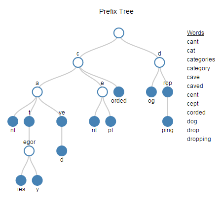
The diagram to the right is an example of a prefix tree. I used the list of words on the right side of the diagram to build this sample prefix tree. In practice you might have a very big prefix tree with many branches and many levels.
Building a prefix tree is half the battle in using edit distances on big data. Once you have your data organized in a prefix tree, you then need to break up your edit-distance algorithm. This is so you can calculate interim values as you walk the prefix tree with your query strings. It’s not too hard to do. I will show you an example in my second post.
So conceptually, you have a prefix tree and you have an edit distance algorithm with interim values. The last thing you need for a big-data solution is some declaration that you will only accept an edit distance no greater than a selected value. For now, let’s use an edit distance of 2. Now, with these tools in hand, you can walk your prefix tree with your query string and your edit distance algorithm, and prune any branches where your minimum interim value is greater than 2. With the right dataset, you will prune many many branches and significantly speed up your query.
Building a prefix tree and walking it with an edit distance algorithm is a relatively simple tasks for lists that fit into memory. There are examples on the Internet for most major programming languages. But what about very large lists? What about a list that’s hundreds of millions of entries long or billions of entries long? What about lists that span multiple computing nodes and won’t fit into memory? Then you need a big data solution and that solution might not be quite so obvious.
There is a naive approach to building a horizontally-scalable prefix tree for very large datasets. For this approach, you take a cumulative hash of each of the characters for each of the entries in your list. Take the word “category” for example. You would push each character of the word through a hash algorithm. As you add each character to the algorithm, you would return each character as a node along with its cumulative hash as an identifier and the cumulative hash of the previous character as a parent id. In this way the path to “t” in the word “category” would be identical to the path to “t” in the word “categories”. Because the paths are the same (“cat”), both would share the same hash id and parent hash id. You would do this independently across multiple compute nodes. From there you would de-duplicate the new list you’ve generated to represent the prefix tree.
The downsides to this naive approach are significant. There are lots of data generated because hash keys are quite large and you need two hash values for each character (node id and parent id). There no opportunity to consolidate nodes without revisiting all of the branches of the tree across all of the computing nodes of your system. Fortunately, there is a better way. It is possible to create consolidated nodes from the start. It is also possible to assign node ids and parent ids without resorting to hash keys. This makes lookups much faster and eliminates volumes of unneeded hash ids.
In the rest of this blog post I focus on doing just that — building optimized horizontally-scalable prefix trees for big data. I demonstrate how to take an initial dataset, identify nodes, and assign node ids. In a follow up post, I will show you how to query a prefix tree on a horizontally-scalable system using an edit distance algorithm. From there, you will be able to apply these techniques to a wide variety of data.
Building Prefix Trees
There are just a handful of distributed operations (8 to be precise) needed to efficiently solve most big-data problems (~95% – 98% of them). As we model our big-data solution together to build our prefix tree, we’re going to focus on two operations. These are Iterate and Normalize. These operations are the work horses around the novel part of our big-data solution.
Iterate processes records in a dataset allowing context between each record.
Normalize processes each record within a dataset multiple times to create multiple records per input record.
These may be new concepts to you or you might associate these words with different meanings. If so, take a moment to review the definitions of iterate and normalize again.
Now let’s take a look at some example data we’ll use to apply these concepts.
| Words cant cat categories category cave caved cent cept corded dog drop dropping |
Notice that the list is sorted. If you compare any two adjacent words you can begin to see where prefixes overlap. We need to turn this observation into a set of rules to build our prefix tree. To identify nodes you need to:
- Start with the first entry. It gets compared to nothing (this is how iterate initializes). The beginning of the first node is where the prefix overlap ends. In this case, the first letter of the first entry is the beginning of a node.
- Move on to the second entry and compare it with the first entry. Carry forward any nodes from the previous step that are present before the beginning of the next node. The beginning of the next node is where the prefix overlap ends.
- Move on to the third entry and compare it to the second. Carry forward any nodes from the previous step that are present before the beginning of the next node. The beginning of a new node is where the prefix overlap ends.
- Continue this way through the list.
- To capture any nodes missed, go through the list again but in reverse order.
Walking Throught the Example
- The first word in the list is “cant”. This word is compared to nothing. That means the first character is where the overlap ends and is the begining of the new node. A new node of our prefix tree is identified below with a “1”.
- The second word “cat” is compared with the first word “cant”. “ca” overlaps in both words. The “t” in “cat” is the end of that overlap. “t” becomes the begining of the new node and any existing nodes in the overlap are brought forward.
- The next two words to be compared are “cat” and “categories”. The first three letters, “cat”, overlap in each word. The “e” in categories is the end of that overlap and is marked as the next node. Any nodes in the overlap are brought forward.
- The process continues throught the word list. The list is first processed in the forward direction. Then the list is processed in the reverse direction to pick up nodes that are identified later in the process.
| Words cant cat categories category cave caved cent cept corded dog drop dropping |
First Pass 1000 101 1011000000 101100001 1010 10101 1100 1110 110000 100 1100 11001000 |
Second Pass (In Reverse) 1010 101 1011000010 101100001 1010 10101 1110 1110 110000 110 1100 11001000 |
Coding a Solution
To code the solution you can use ECL’s iterate operation to compare two entries. From there, you can use normalize to break out all of the nodes from each record. Finally, a dedup operation will get rid of duplicates. If the rest of these operations don’t make sense to you, don’t worry. We’ll go over them in the code example.
The code below simply defines a dataset of words for us to work with and outputs the dataset:
WordLayout := RECORD
   STRING   word;
END;

input_ds:= DATASET([{'cant'},{'cat'},{'categories'},{'category'},{'cave'},{'caved'},
                    {'cent'},{'cept'},{'corded'},{'dog'},{'drop'},{'dropping'}], WordLayout);

output(input_ds, named('input_dataset'));
This next section of code extends the last layout with fields we will need later. We’ll also intelligently set initial values:
NodesLayout := RECORD
   input_ds;
   // The nodes field is where we keep track of when nodes begin.  We're initializing the field to
   // zero fill with the same number of zeros as characters in each word.
   // The extra '1' at the end is a place holder for an end-cap node representing the word itself.
   STRING    nodes        := REGEXREPLACE('.', input_ds.Word, '0') + '1';
   UNSIGNED4 node_cnt     := 0;        // The number of nodes in the word
   UNSIGNED4 compute_node := 0;        // The compute_node this record is on
   DATA      node_ids     := (DATA)''; // Where we pack up the node IDs right before we normalize the prefix tree records
END;
nodes_format_ds := TABLE(input_ds, NodesLayout, UNSORTED, LOCAL);
output(nodes_format_ds, NAMED('reformated_list'));
Below we are using in-line C++ to create a function that will mark where nodes start and end. We are using in-line C++ for maximum portability, but we could have used another language such as Python or Java (The HPCC supports a number of languages). This function will be plugged into the Transform that is part of our first and second Iterate operations:
STRING MarkNodes(STRING l, STRING l_nodes, STRING n, STRING n_nodes) := BEGINC++
   /// This C++ function is designed for use with ECL's Iterate to take a group of
   /// strings and return the prefix tree node structures in a separate field.
   /// The function requires a sorted list and two passes (one in each direction)
   /// l is for the last field, n is for the next field, out is for output
   /// nodes contain the indicator of if we should start a node
   /// An initial value of the node for each field is a string of 0 [zeros]
   /// the same length as the string in question -- an optional 1 can be
   /// added at the end as a word end-cap.
   /// CFK 08/05/2015
   #option pure
   #body
   unsigned long i = 0;

   char * out = (char*)rtlMalloc(lenN_nodes);
   memcpy(out, n_nodes, lenN_nodes);
   while ( i < lenN){
      /// If the characters don't match or
      ///   if we are at the end of the last string then
      ///   flip the 0 to a 1 and break out of the loop
      if (l[i] != n[i] || i >= lenL){
         out[i] = '1';
         break;
      }
      if (l_nodes[i] != n_nodes[i]){
         out[i] = '1';
      }
      i += 1;
   }
   __lenResult = lenN_nodes;
   __result = out;
ENDC++;
Here we are defining our transform to calculate where nodes begin. Also we are counting the number of nodes we find (by counting the “1”s). Finally, we keep track of which compute node is doing the processing (useful information to have for debugging and for later). With the two Iterate operations, we go through the list once in each direction. The second time is to carry back any nodes that got created in the first pass but created later in the list:
NodesLayout GetPTNodesTransform(NodesLayout L, NodesLayout R) := TRANSFORM
   SELF.nodes        := MarkNodes(L.word, L.nodes, R.word, R.nodes);
   SELF.node_cnt     := stringlib.StringFindCount(SELF.nodes,'1');
   SELF.compute_node := Thorlib.Node();
   SELF := R;
END;

pt_nodes_1_ds := ITERATE(SORT(nodes_format_ds, -word, LOCAL), GetPTNodesTransform(LEFT, RIGHT), LOCAL);
pt_nodes_2_ds := ITERATE(SORT(pt_nodes_1_ds,    word, LOCAL), GetPTNodesTransform(LEFT, RIGHT), LOCAL);

output(pt_nodes_2_ds, named('find_pt_nodes'));
Here again we use in-line C++ along with Iterate to help us assign node IDs. Notice that we compare like nodes for finding existing IDs and we use the last ID assigned in the previous record to tell us what the next node ID should be.
STRING AssignNodeIDs(STRING l, STRING l_nodes, UNSIGNED4 l_node_cnt, STRING l_node_ids,
                     STRING n, STRING n_nodes, UNSIGNED4 n_node_cnt, UNSIGNED4 compute_node) := BEGINC++
   /// This C++ function is designed for use with ECL's Iterate
   /// It assigns ID's to prefix tree nodes so that the nodes can later be broken out into
   /// individual records with ECL's Normalize.
   /// CFK 08/05/2015
   #option pure
   #body
   unsigned long long last_node_id = 0;
   unsigned long i = 0;
   unsigned long node_cnt = 0;

      // The new value is empty.
      // Could happen if there are blanks in your word list.
      if (n_node_cnt == 0){
         __lenResult = 0;
         return;
      }

      // Initialize "out" with node ID's from the last iteration
      //  But don't go over if there are too many node ID's from the last iteration
      char * out = (char*)rtlMalloc(n_node_cnt * 8);
      i = (l_node_cnt < n_node_cnt) ? l_node_cnt : n_node_cnt;
      memcpy(out, l_node_ids, i * 8);

      // Find the ID assigned to the last node from the last word.
      //  This will be the starting point to assign new node IDs
      if (l_node_cnt != 0){
         memcpy(&last_node_id, &l_node_ids[(l_node_cnt - 1) * 8], 8);
      }
      else{
         // This is the starting point for node id on each compute node.
         // Setting last_node_id to a value based on the compute node's
         // unique id ensures that each prefix tree built locally on each
         // compute node has unique non-overlapping ID's.  An unsigned long long
         // has a maximum value of 9,223,372,036,854,775,807 or 2^64 - 1.
         // Multiplying compute_node by 10^14 allows for 92,233 compute nodes
         // and 72 Trillion prefix tree nodes on each compute node.  These maximums
         // can be adjusted to fit your needs.
         last_node_id = (compute_node * 100000000000000);
      }

      // Find the first location where the two words don't match
      //  And keep track of how many nodes we've seen
      i = 0;
      while (i < lenL && i < lenN){
         if (l[i] != n[i]){
            break;
         }
         if (n_nodes[i] == '1'){
            node_cnt += 1;
         }
         i += 1;
      }

      // Start adding new node ids to "out" from where we left off
      while (i < lenN){
         if (n_nodes[i] == '1'){
            last_node_id += 1;
            node_cnt += 1;
            memcpy(&out[(node_cnt-1)*8], &last_node_id, 8);
         }
         i += 1;
      }

      // Add the final node id for the end-cap (referenced in comments at the top)
      last_node_id += 1;
      node_cnt +=1;
      memcpy(&out[(node_cnt-1) * 8], &last_node_id, 8);

    __lenResult = n_node_cnt * 8;
    __result    = out;
ENDC++;

NodesLayout GetNodeIdsTransform(NodesLayout L, NodesLayout R) := TRANSFORM
   SELF.compute_node := Thorlib.Node();
   SELF.node_ids    := (DATA) AssignNodeIDs(L.word, L.nodes, L.node_cnt, (STRING) L.node_ids,
                                    R.word, R.nodes, R.node_cnt, SELF.compute_node);
   SELF := R;
END;

node_ids_ds := ITERATE(SORT(pt_nodes_2_ds,  word, LOCAL), GetNodeIdsTransform(LEFT, RIGHT), LOCAL);

output(node_ids_ds, named('get_node_ids'));
Here we use Normalize to break the nodes out into individual records. We use a function to assign our node IDs and parent node IDs to individual records. We will need parent IDs later to query our prefix tree. We use another function to get the node values. Finally we identify if the node represents a full word (what we called an end-cap in the code documentation). This end cap will simplify querying our prefix tree.
PTLayout := RECORD
   UNSIGNED  id;               // Primary Key
   UNSIGNED  parent_id;        // The parent for this node.  Zero is a root node
   STRING    node;             // Contains the payload for this node
   BOOLEAN   is_word;          // Indicates if this node is a word (an end-cap with no children)
   UNSIGNED4 compute_node;     // The compute-node ID this record was processed on
END;

UNSIGNED GetID(STRING node_ids, UNSIGNED4 node_to_retrieve) := BEGINC++
   /// Function returns a numeric node id from a group of node ids
   /// CFK 08/05/2015
   #option pure
   #body
   unsigned long long node_id = 0;
   if (node_to_retrieve != 0){
      memcpy(&node_id, &node_ids[(node_to_retrieve - 1) * 8], 8);
   }
   return node_id;
ENDC++;

STRING GetNode(STRING word, STRING nodes, UNSIGNED4 node_to_retrieve):= BEGINC++
   /// Function returns the substring associated with a node
   /// CFK 08/05/2015
   #option pure
   #body
   unsigned int i = 0;
   unsigned int j = 0;
   unsigned int k = 0;

   // find the start (i) of the node in question
   while(i < lenNodes){
      if(nodes[i] == '1'){
         j +=1;
      }
      if (j==node_to_retrieve){
         break;
      }
      i += 1 ;
   }

   j = i + 1;

   // find the end (j) of the node in question
   while(j < lenNodes){
      if (nodes[j] == '1'){
         break;
      }
      j += 1;
   }

   k = j - i;
   char * out = (char*)rtlMalloc(k);
   memcpy(&out[0], &word[i], k);

   __lenResult = k;
   __result   = out;

ENDC++;

PTLayout NormalizePTTransform(NodesLayout L, UNSIGNED4 C):= TRANSFORM
   SELF.id           := GetID((STRING)L.node_ids, C);
   SELF.parent_id    := GetID((STRING)L.node_ids, C-1);
   SELF.node         := IF(C=L.node_cnt, L.word, GetNode(L.word, L.nodes, C));
   SELF.is_word      := IF(C=L.node_cnt, True, False);
   SELF.compute_node := Thorlib.Node();
END;

/// Break each word record into multiple node records
normalized_pt_ds := NORMALIZE(node_ids_ds, LEFT.node_cnt, NormalizePTTransform(LEFT,COUNTER));

output(normalized_pt_ds, named('normalize_pt_ds'));
Finally, we de-duplicate our results.
final_pt_ds := DEDUP(SORT(normalized_pt_ds, compute_node, id, LOCAL),compute_node, id, KEEP 1, LEFT, LOCAL); output(final_pt_ds, named('final_pt_ds'));
Assumptions About Your Data and Performance
The example code above makes two assumptions about the data in question. It assumes that the data is de-duplicated. It also assumes that the data is distributed so that, as much as possible, adjacent records sit on the same computing node. This keeps duplicate tree nodes to a minimum while taking advantage of the LOCAL key words liberally used in the code above.
The LOCAL keywords tell the HPCC that it can perform certain tasks on each compute node independently without waiting for or coordinating with other compute nodes.
Because of the LOCAL key word, there may be a very small number of duplicate tree nodes in your final prefix tree. These would only occur at the boundary points between two compute nodes. This is handled in the code above by incorporating compute-node IDs into the node IDs of the prefix tree. The code above will work if you take out all of the LOCAL key words above but leaving them in significantly speeds up processing for very large datasets. Ultimately, any duplicates come out in the wash when you search your prefix tree. I’ll cover searching your prefix tree in mynext post where I show how to query a prefix tree on a horizontally-scalable system using an edit distance algorithm, offer performance metrics, and provide code examples for download.
###Update###
Submitted by ckaminski on Sat, 01/07/2017 – 4:15pm
I’ve created a set of function macros that can do the heavy lifting for you. Check them out at https://github.com/Charles-Kaminski/PrefixTree
-Charles