Adventures in GraphLand (The Wayward Chicken)
The other evening I was distracted from a lengthy debug session by a commotion coming from the chicken coop. I raced out the door fearful that some local predator had decided to attempt to steal some dinner. I discovered no such thing; rather ‘the girls’ were all agitating to get out of the coop. In my concentration I had forgotten that it was past the time they are normally allowed out for their daily forage. I immediately opened the coop door and with an explosion of feathers the girls hurtled from the coop in all directions across the yard; each one individually convinced that the particular location that they had chosen to run to was liable to yield the most and tastiest bugs. Last out of the coop stalked our rooster with a grim look on his face; he would be spending the next hour trying to round his charges into the same place so that he could protect them from predators.
This tale of bucolic bliss is not provided to amuse; rather it illustrates the behavior of most programmers when first presented with a graph to analyze. Some deep primal instinct somehow persuades the otherwise analytic mind that the best way to tackle a graph is to scamper all over the place collecting snippets of information as one travels. One of our top technologists responded to my first blog with: “How do I get as far as possible as quickly as possible? Can I go backwards and forwards along the same path? What if I run around in circles? What if I get trapped? How do I know if I wander so far that I’m about to fall off the map?” Being a top technologist his language was rather more erudite (shortest path, directedness, cyclicity, connectedness and centrality) but the intuitive meaning is identical.
I don’t know what causes programmers to do this but I suspect it may be related to the (false) Urban Myth that everyone is related to Kevin Bacon by six degrees of separation. As part of a drastically over affirmed society our take-away from this myth is that there is yet another reason why we are special. I would suggest that if everyone is within six degrees of Kevin Bacon then the correct take-away should be that there is no significance to being within six degrees of Kevin Bacon.
Rather more mathematically; let’s assume that everyone has 25 close associates (relatives, co-workers, neighbors, in-laws) and as a first approximation let’s assume that the graph spans out evenly and without cycles. Then by six degrees of separation you have 25^6 = 240M people; around the adult population of the US. If I were to say: “There are two million criminals in the US, you are in the US, therefore you might be criminal” people would think I were crazy. If I were to say that I had computed that two million of your sixth degree relatives were criminal; then you would be in for questioning. The reality is that the two statements are essentially the same.
Even if we narrow our sites far further, if you view ‘relatives’ as a social network (25 people) rather than pure blood (3-9 people) then by third degree relationships you have fifteen thousand people; you would expect around 150 of them to have done jail time simply by random chance. At a statistical level if your graph has a branching factor of 25 then a fact regarding a second degree relative is twenty five times less significant than one relating to a first degree relative.
As such: the best and most significant information is always close to home.
This insight is one of the core drivers behind the KEL programming philosophy. Whilst some graph languages proudly declare they are ‘graph traversal’ languages; KEL is a knowledge engineering language. Specifically:
KEL exists to concentrate knowledge from the graph into the entity (not to scatter the query from the entity to the graph).
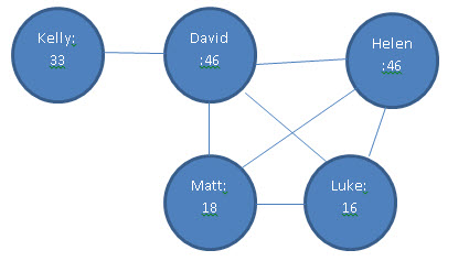
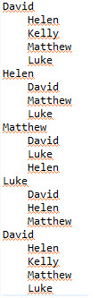
To illustrate the difference I want to tackle a question for the data presented in the last blog: “how many of your first degree relatives are the youngest person they know?” To make this easier to visualize here is the graph:
To answer the given question for ‘David’ here is a plausible graph traversal approach:
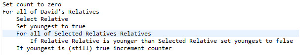
If you execute the above you will visit the following nodes in sequence:
So a query about David causes us to visit 15 nodes. As an exercise, you should try writing out the nodes visited if I wanted to know the average number of youngest relatives for the two oldest people in the graph. You should visit 29 nodes.
The KEL methodology is rather different:
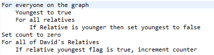
Pleasingly it is rather easier to read in KEL than it is in pseudo-code!
Person: => Youngest := COUNT(Relationship(whoelse.Age<Age))=0;

Person: => YoungRels := COUNT(Relationship.whoelse(Youngest));
This is not a language tutorial but there are a couple of aspects of the above worth noting:
- The ‘Person:’ defines the scope of the operation. It applies to Person nodes.
- The space between the ‘:’ and the ‘=>’ allows a precondition for the operation to apply; that will be a later subject.The interesting piece occurs after the ‘:=’ so we will look at the first in detail:
So,
COUNT(Relationship)
in the person scope would give you the number of relationships for each person.
For this particular computation we want to filter those associations further, to those in which the OTHER person in the relationship is younger. We do this using: (whoelse.Age<Age). If there is no-one who is younger than you are then you are declared to be the youngest.
Subsequent to this line every Person node has a new property available ‘Youngest’ which can be queried as used as any other property. Thus in the second line, we can compute the number of youngest relatives simply by counting and using the Youngest property as a filter.
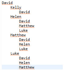
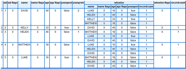
The nodes visited to compute the query for David are:
Er, which is 22! That is 7 more visits that the normal method! Why would I go to such pains to make my life harder? Well, now trace through how many extra visits do I have to make to compute the average of the two oldest people? The total should be 26; a savings of 3. Now suppose I want to know the average number of youngest relatives across the whole graph; suddenly the KEL solution begins to pull substantially ahead.
So what is happening? In the traditional model, each computation for each entity moves away from the entity to the first degree relatives which in turn have to move to their first degree relatives to compute the answer. Thus most of the computations are performed at the second degree from the original entity being considered.
If viewed programmatically, within the KEL model this second degree query is written as two subsequent first degree queries. Of course, the KEL compiler may or may not choose to execute the query that way, and it will almost certainly have different strategies for thor and roxie; but logically that is how it is specified.
We should not however, view KEL programmatically. Rather we should view KEL, or at least the KEL logic statements, as a graph annotation model, or better a knowledge concentration model. With each logic statement, knowledge that could be gleaned by traveling away from a node is moved and stored within the node itself. Queries then execute against the knowledge rich graph that is produced.
There are, of course, examples when a graph query cannot be decomposed into a succession of simpler queries. Those are slightly harder to code and significantly harder to execute; they will be the subject of a later blog. For now just keep in mind; if you can code it as a succession of near-relative encounters then you should do so. In the mean time we need to tackle heterogeneity; what do you do if not all of your entities are the same type? That will be the subject of our next blog.
In closing I would like to present our full ‘program’ as we have it so far; and the answers:
Person := ENTITY(FLAT(UID,Name,INTEGER Age));

Relationship := ASSOCIATION(FLAT(Person who,Person whoelse));
USE File_Person(FLAT,Person);
USE File_Relat(FLAT,Relationship(who=person1,whoelse=person2)
,Relationship(who=person2,whoelse=person1));Person: => Youngest := COUNT(Relationship(whoelse.Age<Age))=0;
Person: => YoungRels := COUNT(Relationship.whoelse(Youngest));QUERY:Dump1 ,Relationship.whoelse{Name,Age,Youngest}};
Produces:
Incidentally: if anyone has the time and inclination to tackle these queries in alternate graph languages I would be very interested to see the results. I would also love to see if someone wants to have a swing at this in ECL; it will help me keep the KEL compiler writer on its toes.

Adventures in Graphland Series
Part I - Adventures in GraphLand
Part II - Adventures in GraphLand (The Wayward Chicken)
Part III - Adventures in GraphLand III (The Underground Network)
Part IV - Adventures in GraphLand IV (The Subgraph Matching Problem)
Part V - Adventures in GraphLand (Graphland gets a Reality Check)
Part VI - Adventures in GraphLand (Coprophagy)