HPCC Systems Causality Toolkit Version 2.0
Overview
HPCC Causality version 2.0 is a major extension to the previous version 1.0. It provides a rich visualization framework as well as other features that make it easier to use, more flexible and more powerful.
In particular, Version 2.0 supports the following new capabilities:
- Visualization – A set of plots to help understand the dataset from both a probabilistic and a causal perspective
- Natural Queries – A simple text based query mechanism allows specification of complex queries in a natural statistical language, rather than formatting complex nested data structures.
- More Data Types – Support for textual as well as numeric data. Dataset can be any mixture of Continuous, Discrete Numeric, Discrete Text, Categorical Numeric, or Categorical Text.
- Probability Sub-Spaces — Used to filter the dataset and to construct conditional multivariate distributions.
- Enhanced Algorithms – Various algorithms have been improved using machine learning and other powerful analytic techniques.
Contents
The HPCC Causality Bundle provides four sub-systems:
- Synth — Allows the generation of complex synthetic datasets with known causal relationships, using structural equation models. These can be used with the other layers of this toolkit or with other HPCC Machine Learning bundles.
- Probability — Provides a rich probability analysis system, supporting conditional probabilities, conditionalizing, independence testing, and predictive capabilities.
- Causality — Provides a range of Causal Analysis algorithms. This layer requires a Causal Model, which combined with a dataset, allows questions to be asked that are beyond the realm of Statistics. Specifically, this module allows: Model Hypothesis Testing, Causal Analysis, Causal Metrics, Counterfactual Analysis (future), and limited Causal Discovery.
- Visualization — Visualize probabilistic and Causal relationships. Provides a range of Plots showing probabilities, joint probabilities, conditional probabilities, and causal relationships.
Setup
Installation
This bundle requires python3, PIP, and “Because” on each HPCC Systems Node
Installing Because
Clone the repository https://github.com/RogerDev/Because.git
Run: sudo -H pip3 install
Example: sudo -H pip3 install ~/source/Because
This must be done on each HPCC Systems Cluster node. It is important to use sudo so that the bundle is installed for all users. Since HPCC Systems nodes run as special user hpcc, installing as the current user would not allow the module to be found by hpcc.
Installing HPCC_Causality
On your client system, where HPCC Systems Client Tools was installed, run “ecl bundle install https://github.com/hpcc-systems/HPCC_Causality.git”.
Getting Started
The first step after installation is to create or load a dataset to be analyzed. The next two sections describe how to load a dataset from a CSV file, or an existing Thor dataset, and how to create a synthetic dataset. If you have a dataset to explore, follow the instructions in Loading your dataset below. If you would like to create a synthetic dataset for exploring the toolkit, skip that section and go to Creating a Synthetic Dataset.
Loading Your Dataset:
You may have a dataset that you would like to work with or may want to start with synthetic data. This section describes how to load an existing dataset, either a Thor dataset, or a CSV file. For an explanation of synthetic data generation, please see Synthetic Data section at the end.
Dataset Preparation
It is often prudent to pre-process a dataset to make analysis more effective. Specifically, we recommend the following:
- Remove any descriptive or nominal variables — Variables containing long text strings of descriptive information or nominal variables such as names, addresses, phone numbers, etc. don’t lend themselves to statistical analysis, and their presence can slow down processing and consume more memory unnecessarily. The useful variables for analysis are numeric variables, and textual variables with non-unique values (i.e., categorical variables).
- Organize textual variable values so that they form a natural order when sorted. For example, our sample dataset has a variable called genhealth (general health). The raw values were: poor, fair, good, verygood, and excellent. If we tried to analyze that variable, we would not be able to determine the natural order. So, we relabeled the values as 1-poor, 2-fair, 3-good, 4-verygood, 5-excellent. Now they will always sort in a meaningful order, and we can treat it similar to numeric data. If a variable does not have a natural order, such as ‘state’ of residence, then note that those should be marked as ‘categorical’ (discussed later). Binary variables with only two values such as yes / no do not need to be relabeled, as either order is fit for analysis.
Loading a CSV File
In this example, we will use a file called llcp.csv that contains a rich set of health survey information.
- Upload the file to a Landing Zone *.
- Import (i.e., Spray) the file as Delimited *.
- Check the box labeled Record Structure Present (assuming that the first line of the CSV contains the field names).
- Go to Logical Files and select the sprayed file (e.g., llcp.csv).
- Go to the ECL tab for that file and copy the record structure there.
- Paste the structure into your ECL program, and assign it to an attribute (e.g., MyFormat).
- The structure will show all fields as STRING type. Edit the structure to make all numeric fields either INTEGER or REAL.
- Load your dataset using:
MyDS := DATASET(‘llcp.csv’, MyFormat, CSV(HEADING(1)));
// Note: The HEADING(1) will cause the field names line to be omitted from the data.
* See HPCC Systems Platform documentation for details on using platform tools.
Loading an Existing Thor File
In this case, you will already have a format.
MyDS := DATASET(‘llcp.flat’, MyFormat, THOR);Creating a Synthetic Dataset
HPCC Systems Causality’s Synth Subsystem allows the creation of rich multivariate datasets with known causal relationships. This allows you to assess the power and limitation of the various algorithms where you already know the correct answers. Synthetic datasets are created using a Structural Equation Model (SEM), that describes how each variable is constructed, and how the variables are inter-related. The resulting dataset is typically a stochastic dataset with defined statistical characteristics. The SEM can be arbitrarily complex, but it is quite easy to get started with simpler models. The Synth module is described in the section Synthetic Data Subsystem below. Here we provide a fairly simple SEM as an example.
IMPORT HPCC_Causality AS HC;
// Define your SEM.  A SEM has 3 parts: Initialization, Variable Names, and the list of equations.
// SEM should be a Dataset Row
MySEM := ROW({
              [], // No initializations for this example
              ['A', 'B', 'C', 'D'], // Variable Names
              // List of equations, as strings
              ['B = normal(2, 3)', // B is normally distributed mean:2, std:3
               'A = .75 * B - 1.5 + logistic(0,.5)', // A is a linear function of B with additive logistic noise
               'D = tanh(2 * A) + exponential(1.0)', // D is a non-linear functon (Hyperbolic Tangent) of
                                                    // A with additive exponential noise
               'C = .5 * B + .5 * D + uniform(-.5, .5)' // C is a linear function of C and D, with uniform
                                                       // noise on the interval [-.5, .5]
               ]});

// Generate 10,000 samples from the defined distribution.
generator := HC.Synth(MySEM); // Create a generator
MyDS := generator.Generate(10000); // Generate the samples
// MyDS is now a dataset ready to use.
Analyzing Your Dataset
Analyzing your dataset always starts with the Probability sub-system. The Visualization and Causality Subsystems utilize Probability Spaces that have been created by Probability.
Import HPCC Causality
IMPORT HPCC_Causality AS HC;Load your data into a Probability Space
- Define which variables are categorical, if any. The system cannot determine whether a variable is categorical, so you must tell it. Categorical variables are variables with more than two possible values, where there is no natural order to the values. For example, in our dataset, state, and smokertype are considered categorical.
Categoricals := [‘state’, ‘smokertype’];- Several macros are provided to convert your dataset into a form that can be used by Probability.
// Add a sequence id to each record.  IDs must be sequential from 1 to N (the number of records).
// Note: Macros do not return a result.  The result is placed into the attribute named by the second parameter.
HC.AddID(MyDS, MyDS2);

// Convert the data into a cell-based format that supports both textual and numeric data.
// Note that this macro also produces an attribute <output_attr>_fields (e.g. MyDSFinal_fields) that contains
// the field names in the correct order.
HC.ToAnyField(MyDS2, MyDSFinal);

// Now load the data into a probability space:
prob := HC.Probability(MyDSFinal, MyDSFinal_fields, Categoricals);

// At this point, you can request a summary of the loaded dataset, which shows the number of records loaded,
// the fields, and the detected values for each field.
summary := prob.Summary();
OUTPUT(summary, NAMED(‘DatasetSummary’));
Once we have a Probability Space (i.e., prob), we can use that in any of the three analytic subsystems: Probability, Visualization, or Causality.
All of the analytic subsystems utilize a common Probability Query Language (PQL). This is, for the most part, a natural mathematical language, consistent with textbook probability expressions. We describe the basic PQL in the next section. The Subsystem Details section will discuss subsystem-specific variants.
Probability Query Language
A wide range of probability queries are supported. Queries are formatted as strings in natural statistical terms. The general form is:
P(<target> | <conditions>), read: ‘The probability of the target expression given the conditional expression’.
A target expression may be a bare variable name which refers to the variable as a whole or a comparison of a variable to a value or set of values. The former is referred to as an ‘unbound’ variable, and the latter a ‘bound’ variable. In some cases multiple bound variables can be used in the target, which represent a ‘joint probability’. The variable expressions are separated with commas. Likewise, the conditions can be one or more bound or unbound variable expressions separated by commas. Each query is a single string, with no internal string quotations necessary for variable names or string values. The parser automatically detects string literals.
The following comparators can be used for bound variables within a query. They can be used with both textual and numeric values. Textual value comparisons use the alphabetical order of the values for ordinal comparison.
- variable = value — Equality.
- variable > value — Greater than.
- variable >= value — Greater than or equal to.
- variable < value — Less than.
- variable <= value — Less than or equal to.
- variable between [value1, value2] — Variable is greater than or equal to value1 and less than value2.
- variable in [value1, … , valueN] — Variable in a set of values.
The remainder of this section looks at how PQL is used in each of the analytic subsystems.
Probability Queries
// Numerical Queries of Probability values or Expectations.
queries := [
            // The probability that a survey participant’s age is greater than or equal to 65
            ‘P(age >= 65)’,
            // The probability that general health takes on one of the 3 indicated
            // text values, given that a person’s age is between 65 and 80.
            ‘P(genhealth in [3-good, 4-verygood, 5-excellent] | age between [65, 80])’,
            // The expectation of income for individuals whose health is poor.
            ‘E(income | genhealth=1-poor)’
            ];

// Issue the set of queries and output the result.
qresults := prob.Query(queries);
OUTPUT(qresults, NAMED(‘NumericalQueries’));

// We can also query for distributions.  For distributions, the probability target (i.e. the first clause of the query)
// should only contain a single bare variable (i.e. an unbound variable).  This indicates that we are talking about
// the full distribution of the variable.  Distribution queries return a distribution structure, detailing
// characteristics of the distribution in question.
dqueries := [
             // The distribution of the variable 'height'.
             ‘P(height)’,
             // The distribution of height for females.
             ‘P(height | gender=female)’,
             // The distribution of weight for males 65 or older.
             ‘P(weight | gender=male, age >= 65)’,
             // The distribution of income for males when we control for age in the sample.
             // Note that an unbound variable in the condition implies conditionalization
             // (i.e. controlling-for) in probabilistic and causal queries, but has a slightly
             // different meaning for visualization.
             ‘P(income | gender=male, age)’,
             // An alternate expression of the previous query.
             ‘P(income | gender=male, controlFor(age))’
            ];

// We use QueryDistr when we are looking for distributions to be returned, since distributions are
// very different from the single values returned from bound targets or expectations as above.
dqresults := prob.QueryDistr(dqueries);
OUTPUT(dqresults, NAMED(‘DistributionQueries’);
Causal Queries
The Causality module provides a range of Causal algorithms. Causality operates above the Statistical (i.e., Probability) level, and requires a Causal Model that describes the graph of causal relationships between variables. With a Causal Model, the causal algorithms can support queries that cannot be expressed at the level of Probabilities. Causality provides a way to describe the Causal Model, and a set of algorithms to discover a Causal Model from the data. Because the causal signals are very subtle, it is not always possible to accurately discover the correct Causal Model. It is anticipated that the user will combine the discovered information with domain knowledge to build the best Causal Model. The closer the Causal Model is to the ground truth, the more accurate will be the queries and inferences produced by Causality.
Causal Models are specified by listing the causes of every non-exogenous variable. Exogenous variables are variables that come from outside the model and do not have any causes within the model. In the example below, we use the classic model of Temperature effecting both Ice Cream consumption and Crime. The model is described by listing each variable and its causes.
IMPORT HPCC_Causality AS HC;
Types := HC.Types;

// Describe each RV and its causes. RV = Random Variable.
RVs = DATASET([
               {'Temperature', []}, // Exogenous
               {'IceCream', ['Temperature'], // Ice Cream consumption is effected-by Temperature
               {'Crime', ['Temperature', 'IceCream'] // We hypothesize that both Temperature and Ice Cream
                                                     // may affect Crime.  We can then test that hypothesis.
               ], Types.RV);
// Now make a causal model out of the list of RVs
MyModel := DATASET({'MyModelName', RVs}, Types.cModel);
Causality supports queries that are a superset of Probability queries. Any probability query will return the same results through Causality as it did through Probability. In addition, Causality supports Causal Interventions, which can only be computed in the presence of a Causal Model. This is expressed using a do(…) semantic that is added to the conditions clause of the query. Within the do(…) clause, a set of interventions can be expressed as <variable> = <value>. For example:
‘P(diabetes = yes | do(exercise=no), age > 65)’ — The probability of a person over 65 having diabetes, while intervening to prevent them from exercising.
Note that in the example above, we are not asking the probability of a person over 65 who doesn’t exercise having diabetes. The do() intervention analyzes the data so as to distinguish remove non-causal correlation and remove it from the calculation. So if we assume that age and exercise are correlated, this query would yield different results from the probabilistic query: ‘P(diabetes = yes | exercise=no, age > 65’). This allows true causal effects to be observed. By comparing the above query with its alternative: ‘P(diabetes = yes | do(exercise=yes), age > 65)’, we can directly discern the effect of exercise on diabetes for people over 65. At the Statistical level, the only way to calculate this is to run a Randomized Controlled Experiment where each participant is (randomly) required to either exercise or not — an experiment that would be impossible (and unethical) to implement in a free society.
// Does Ice Cream Consumption have an effect on crime???
// Let's create a synthetic dataset simulating this scenario
semRow = ROW({
              [], // Initializers not used
              ['Temperature', 'IceCream', 'Crime], // Our three exposed variable names
              [
                 'ce = 0.0', // This lets us vary the causal effect in the simulation 0.0 = no effect
                 'Day = round(uniform(0, 364))', // Pick a day of year for this observation.
                 'Temperature = sin(Day / (2*pi)) * 30 + 40 + normal(0, 5)', // Pseudo-realistic seasonality:
                                      // Temp varies +/- 30 by season with mean 40, and daily fluctuations
                                      // normally distributed with std of 5.
                 'IceCream = 1000 + 10 * Temperature + normal(0,300)', // Simulate IceCream consumption.
                 'Crime = ce * IceCream + 50 + 3 * Temperature + normal(0,2)' // Simulate Crime.
               ], Types.SEM);

// Generate 10,000 samples.
mySEM := = DATASET([semRow], SEM);
simData := HC.Synth(mySEM).Generate(10000);  // 10,000 observations

// Create the probability space
prob:= HC.Probability(simData, semRow.varNames);

iHigh := 1700;  // A high level of Ice Cream consumption
iLow := 1300;  // A low level of Ice Cream consumption
// We measure the expectation of Crime when we intervene on IceCream, setting it to iHigh, and to iLow.
queries := [
          'E(Crime | do(IceCream=' + (STRING)iHigh + '))',
          'E(Crime | do(IceCream=' + (STRING)iLow + '))'
           ];
// Create a Causality instance. Pass it the model (from previous code block), and the Probability Space Id (PSID) from
// the prob module.
psid := prob.PS; // Get the psid from our previously created probability space
cg := HC.Causality(MyModel, psid);

// cg is a causal graph or causality instance.
// It supports Query and QueryDistr commands just like Probability, but with extended syntax.
results := cg.Query(queries);
OUTPUT(results, NAMED('ExperimentResults'));

// If results[1] is not substantially different than results[2], we can reject
// the hypothesis that IceCream consumption affects crime.
Visualizations
Visualizations take the form of 2-dimensional or 3-dimensional plots. Plots show up in ECL Watch under the Resources tab for the work unit.
Visualizations use the same query mechanism as probability queries with a few minor differences. The main difference is that unbound variables in the conditions clause imply plotting against all values of those variables on the independent axes (x for 2D, or x and y for 3D). The controlFor(…) expression must be used to indicate control variables so that they are not mistaken for axis variables. Each plot is defined by a query string, and the plots are invoked using the Viz.Plot() macro:
// We create a list of queries, 1 per plot.  The queries to use for each type of plot are described below.
plotQueries := [
                // Queries go here.  Any combinations of the visualization queries defined below may be
                // included.
                ];

// In order for Viz to find the right probability space, we pass it the Probability Space ID (PSID) that we retrieve
// from our prob module.
// Note that Plot can only be called once in a work unit, so all desired plots should be included in plotQueries.
psid := prob.PS;
HC.Viz.Plot(plotQueries, psid);
Plots show up in ECL Watch under the Resources tab for the work unit.
Let’s look at a few different types of visualization.
Probability Distribution Plots
Probability Plots plot the familiar probability distribution function, such as a bell curve for normally distributed data. They also include variance bars that indicate the width of the distribution. Since plots are limited to 3 dimensions, and a single variable PDF requires 2 dimensions, probability plots are limited to a single conditional variable.
‘P(age)’ – A 2D plot showing the probability distribution function of the age variable.
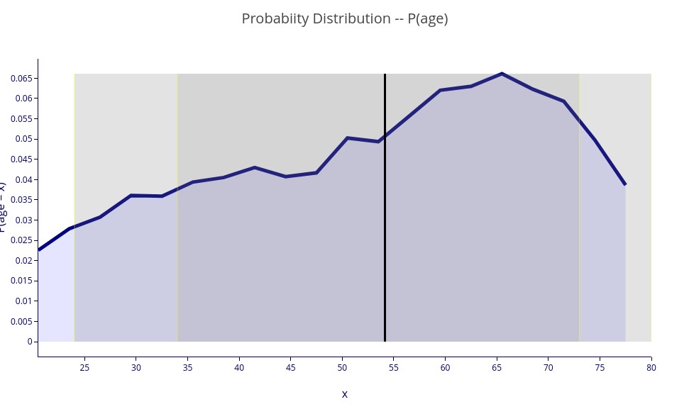
Note that the variance bars (vertical shading) indicate the width of the distribution. Rather than showing standard deviations, that only really make sense for symmetrical distributions, we show the equivalent of one and two standard deviations, but using quantile calculations that apply to asymmetric distributions (like above) as well. The dark bars correspond to 68 percent of the samples (equivalent to one standard deviation, whereas the lighter bars encompass 95 percent of the samples, equivalent to two standard deviations.
‘P(weight | height)’ – A 3D plot showing the probability distribution of weight for each height.
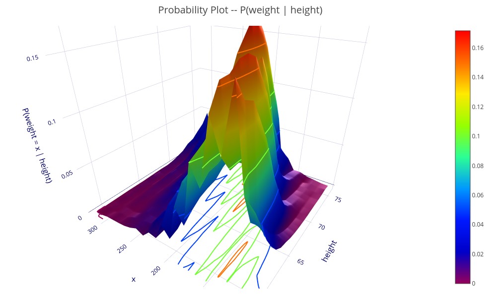
3D plots, shown on the ECL Watch interface can be rotated and zoomed, which is necessary to really understand the complex relationships shown.
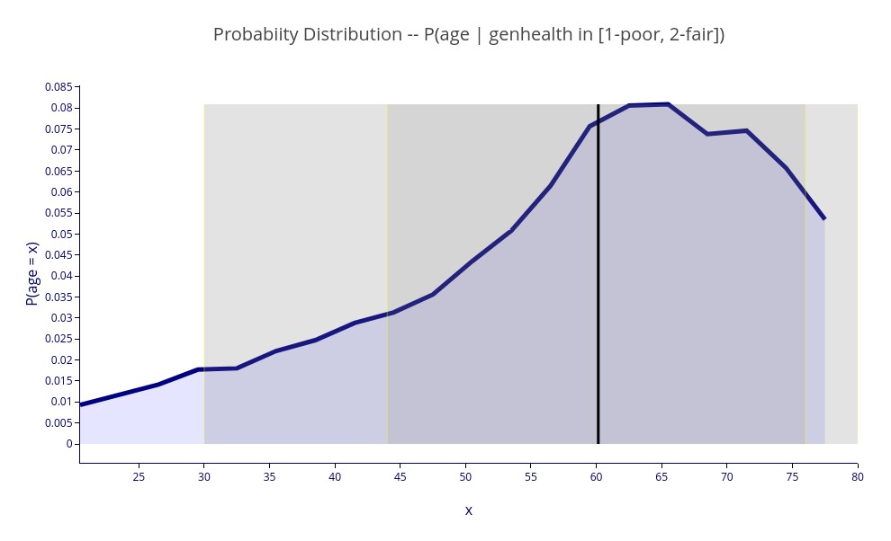
Additional conditions can be used, but must be bound (i.e., include a variable and comparison), in which case they act as a filter.
‘P(age | genhealth in [1-poor, 2-fair])’ – A 2D plot of the distribution of age for respondents with poor or fair health.
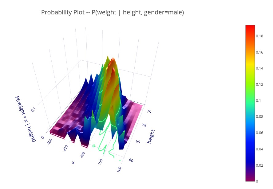
‘P(weight | height, gender=male)’ – A 3D plot showing the probability distribution (for males) of weight for each height.
Expectation Plots
Expectation plots show the expected value (e.g., mean) of a target variable against the values of one or two conditional variables.
‘E(weight | height)’ – A 2D plot showing the expectation of weight for each value of height.
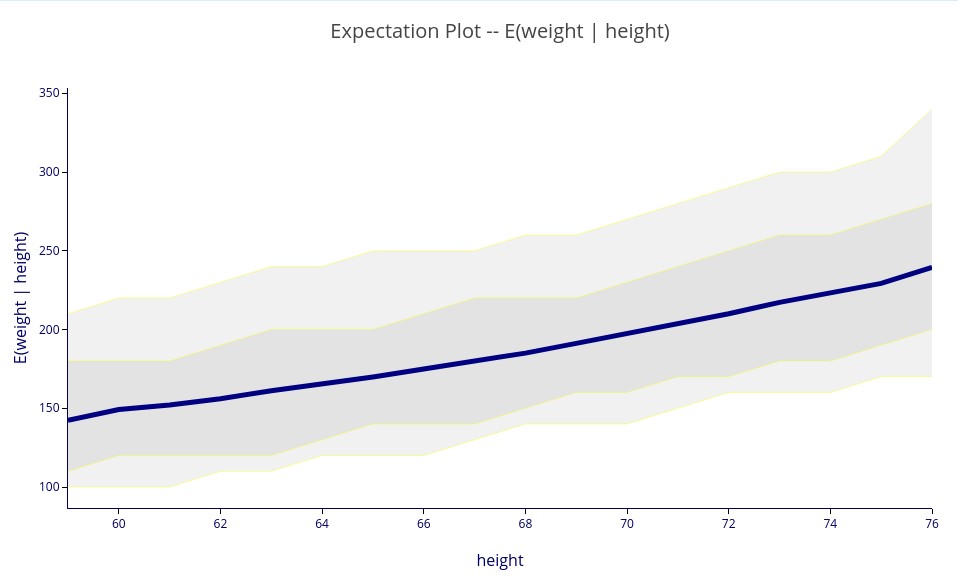
As in probability distribution plots (above), the light and dark bands use quantization levels to approximate one and two standard deviation bands, but for (potentially) asymmetric distributions. You can see in the chart above that the upper bands extend far further than the lower bands, meaning that the distribution is asymmetrical (i.e., skewed) for all values of height.
As with probability plots, additional filtering can be provided by adding bound conditions.
‘E(weight | height, gender=male)’ — Same as previous, but only includes males.
‘E(weight | height, age)’ – A 3D plot showing the expectation of weight for each value of height and age.
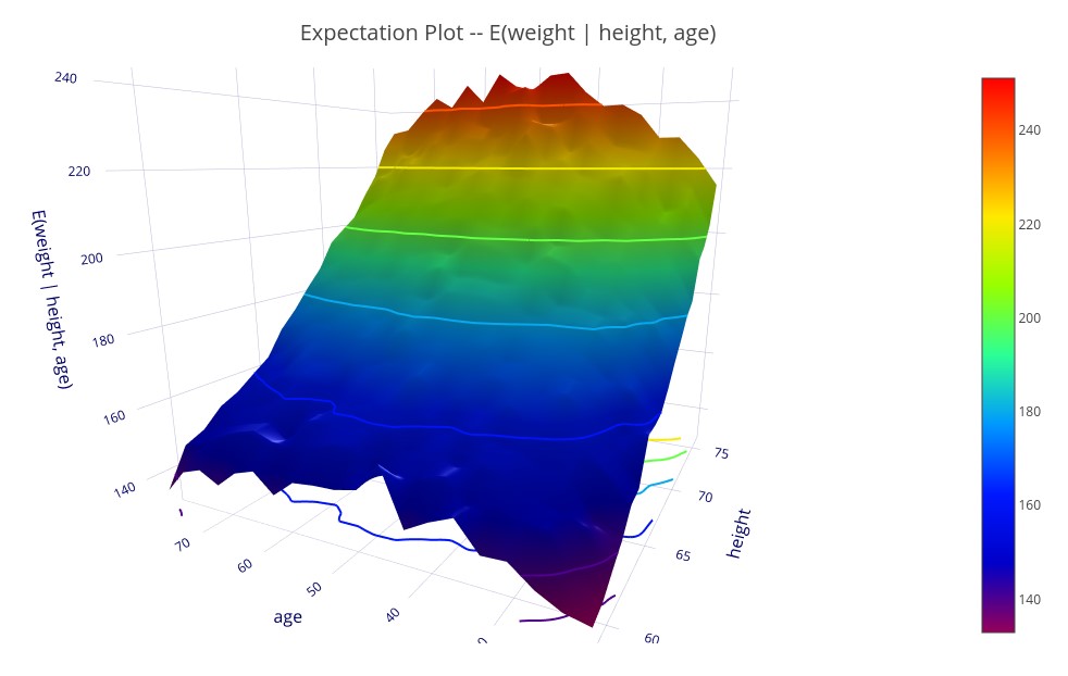
Expectation plots also allow control variables.
‘E( genhealth | state, controlFor(age, income))’ – Expectation of general health level given the state of residency and controlling for variations in age and income between states.

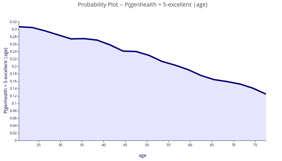
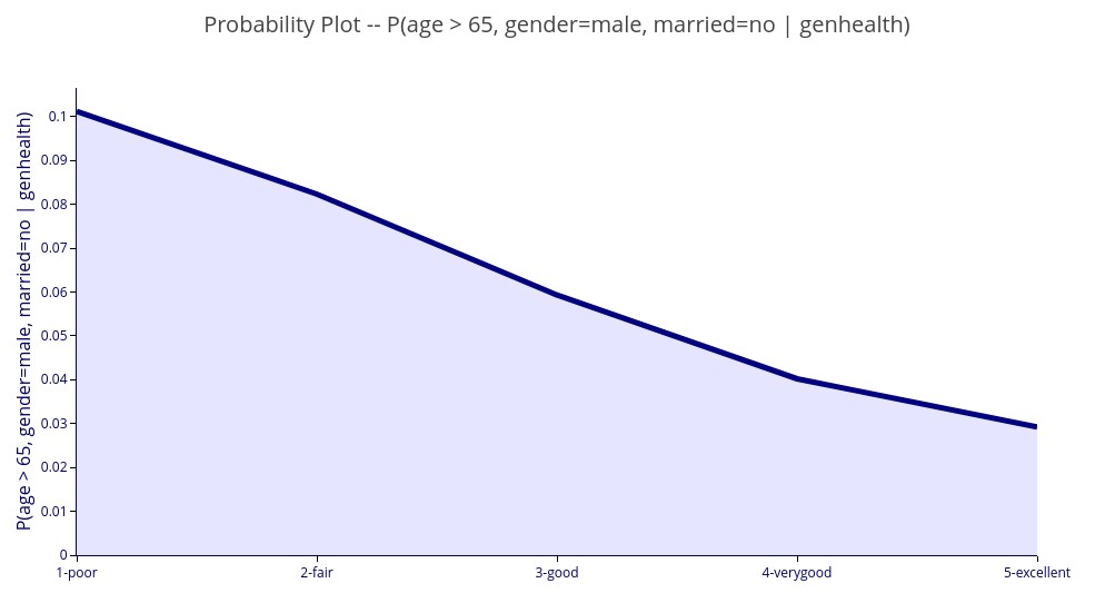
Bound Probability Plots
Bound Probability Plots plot a probability expression given one or two conditions.
‘P(genhealth = 5-excellent | age)’ – 2D plot showing the numerical probability of excellent health for each value of age.
‘P(genhealth in [3-good, 4-verygood, 5-excellent] | age, income) )’ – 3D plot showing the probability of good to excellent health for each value of age and income.
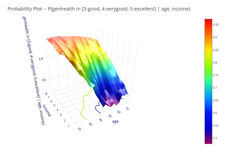
Bound probability plots can specify multiple target variables, in which case it represents the joint probability of all of the target conditions being met.
‘P(age > 65, gender = male, married =no | genhealth)’ – 2D plot of the probability that a person is a male, unmarried, and over 65 years old for each value of general health.
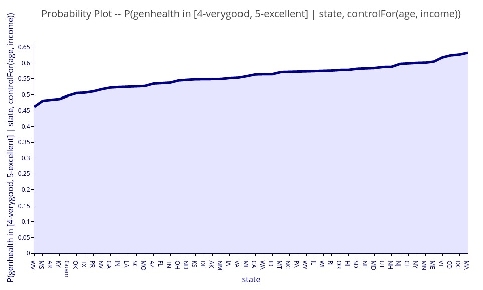
Control variables can also be used.
‘P( genhealth in [4-verygood, 5-excellent] | state, controlFor(age, income))’ – The probability of very good or excellent health for each state of residency and controlling for variations in age and income between states.
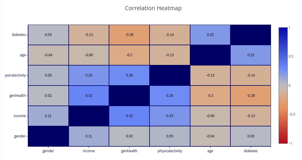
Variable Relationship Heatmaps
Two types of heatmap are supported for understanding relationships between sets of variables: Correlation Heatmaps and Dependency Heatmaps.
Correlation is a linear phenomenon, while Dependency also encompasses non-linear relations. Correlation has a direction (positive or negative correlation) and a strength, while Dependency only has a strength.
These queries are different from the various probability queries in that they do not take any conditions.
‘CORRELATION(gender, income, genhealth, exercise, age, diabetes)’ – A heatmap matrix showing Correlation between each pair of named variables. Blue colors represent positive correlation while orange colors represent negative correlation. The darker the color, the stronger the (positive or negative) correlation.
‘DEPENDENCE(gender, income, genhealth, exercise, age, diabetes)’ – A matrix showing Dependence between each pair of named variables.
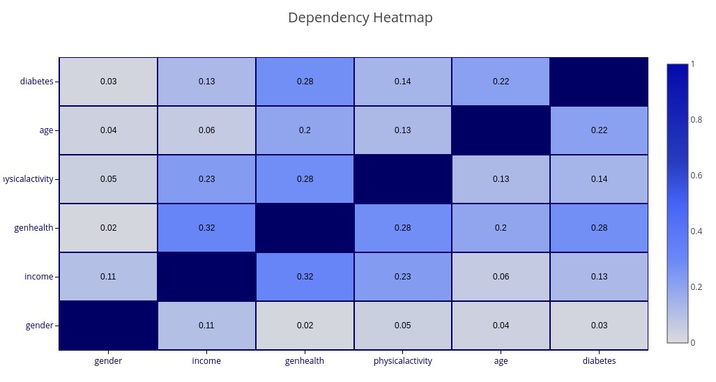
Notice that
If no variables are selected, then all variables (up to 20) will be shown.
Causal Model Plot
The Causal Model Plot runs a causal discovery on the selected set of variables, and plots the model, showing the causal interactions between variables, along with their strength. Causal Discovery attempts to eliminate spurious correlations and leave only the actual causal relationships.
‘CMODEL(gender, age, income, height, weight, exercise, education, genhealth)’ — Generate a 2D graph of the indicated variables and their causal relationships.
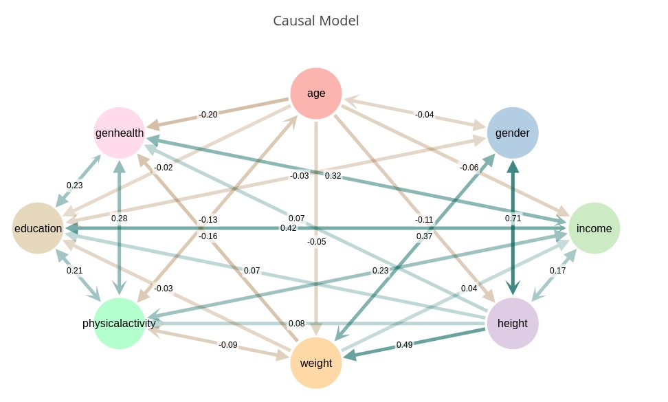
Notice that this causal model is nearly fully connected. This is due to the nature of our survey data that has subtle dependencies between nearly all variables. The dependency algorithms used in Causality 2.0 are extremely sensitive to dependence. We can correct for this using some special tuning parameters.
CModel supports three special tuning variables $power, $sensitivity, and $depth that can be specified in the conditional clause.
$power is a number from 0 to 100 that provides a tradeoff between discriminative power and performance. A value of 0 should discriminate linear relationships, while higher values will discriminate subtler non-linearities. Generally, a value of 3 to 10 is sufficient. If not specified, the default is 5.
$sensitivity range [1.0, 10.0] allows detuning of sensitivity to dependence. The default is 10.0, which indicates maximum sensitivity. In datasets such as our example survey we find that reducing the sensitivity to 5 or 6 provides more useful results. If too many causal links are detected (e.g. , detuning the sensitivity will create a sparser model.
$depth range [1, 5] determines how deeply independencies are explored. Increased depth significantly increases runtime, and with limited data size yields little additional benefit due to the exponential data requirements for dependence testing with high conditional dimensions. Default is 2. Higher values may be productive in some environments.
We correct for the excess connectedness by turning down the sensitivity, which defaults to 10 (i.e., maximum sensitivity). In this case we turn the sensitivity down to 6 and get a more reasonable causal model.
‘CMODEL(gender, age, income, height, weight, exercise, education, genhealth | $power=8, $sensitivity=6, $depth=3)’
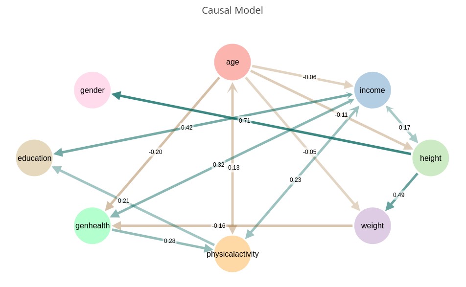
Note that not all of the connections make sense. For example, although we detected a causal relationship between gender and height, we got the direction wrong. This is the nature of the state-of-the-art in causal discovery. One should expect a discovered model to need some degree of tuning based on domain knowledge. The corrected model can then be fed into Causality before retrieving metrics or performing causal inference.
Notice that some connections have arrowheads on both sides. This represents uncertainty as to the causal direction. The straight arrowheads are the inferred direction, while the stylized curved arrowheads represent the uncertainty of the direction. If the curved arrowhead is smaller than the straight one, it implies that we have more confidence in the direction than if they are both the same size, which is a toss-up.
Subsystem Details
See User Documentation for interface details.
Probability Subsystem
The Probability Subsystem provides a wide range of probability and statistical functions.
Module Instantiation:
IMPORT HPCC_Causality AS HC;

prob := HC.Probability(myDataset, varNames, categoricalNames);
Creating a Probability SubSpace:
SubSpace — Create a probability SubSpace with a filter and a parent space.
// Create a new subspace of males in good to excellent health
newPSID := prob.SubSpace('gender=male, genhealth in [3-good, 4-verygood, 5-excellent]', prob.PS
‘Natural’ Probability Queries:
Query — Query for probabilities or expectations using natural query language.
queries = ['P(age >= 65)', 'P(weight > 200 | geneder=male, age between [30, 40])', 'E(weight | height=66, gender)'];
results := prob.Query(queries, prob.PS)
QueryDistr — Query to retrieve univariate distributions of selected variables.
queries = ['P(age)', 'P(weight | height between [60, 80])', 'P(income | gender=female, state=MA)'];
distributions := prob.QueryDistr(queries, prob.PS);
Structured Probability Queries:
Structured queries are more difficult to compose, but may lend themselves to programmatic composition.
P — Structured query for numerical probabilities
E — Structured query for numerical expectations
Distr — Structured query for distributions
IMPORT HC.Types;
ProbQuery := Types.ProbQuery;
ProbSpec := Types.ProbSpec;

// See Types for formatting details.  These are the same queries as for Natural Queries above.

// Probabilities
pQueries := DATASET([{1, DATASET([{'age', [65, 999]}], ProbSpec), DATASET([], ProbSpec)},
                  {2, DATASET([{'weight', [200, 999]}], ProbSpec), DATASET([{'gender', [], ['male']},
                                            {'age', [30,40]}], ProbSpec)}
                   ], ProbQuery);

probs := prob.P(pQueries, prob.PS);

// Expectations
eQueries := DATASET([{2, DATASET([{'weight'}], ProbSpec), DATASET([{'height', [66]},
                                            {'gender'}], ProbSpec)}
                   ], ProbQuery);
expects := prob.E(eQueries, prob.PS);

// Distributions
dQueries := DATASET([{1, DATASET([{'age'}], ProbSpec)},
                  {2, DATASET([{'weight'}], ProbSpec), DATASET([{'height', [60, 80]}], ProbSpec,
                  {3, DATASET([{'income'}], ProbSpec), DATASET([{'gender', [], ['female']},
                                            {'state', [], ['MA']}], ProbSpec)}
                  ], ProbQuery);
distributions := prob.distr(dQueries, prob.PS);
Dependency Testing:
Dependence — Determine the likelihood that two variables are dependent (i.e., not Independent). Returns a number [0.0, 1.0] approximating the probability of dependence. Values greater than .5 indicate probable dependence and less than .5 probable independence. Values around .5 indicate uncertainty.
isIndependent — Returns a boolean indicating if a pair of variables are independent.
dependences := prob.Dependence(DATASET([
                  {1, DATASET([{'age'}, {'income'}], ProbSpec)},
                  {2, DATASET([{'weight'}, {'height'}], ProbSpec),
                  {3, DATASET([{'gender'}, {'diabetes'}], ProbSpec)
                  ], ProbQuery), prob.PS));

boolResults := prob.isIndependent(DATASET([
                  {1, DATASET([{'age'}, {'income'}], ProbSpec)},
                  {2, DATASET([{'weight'}, {'height'}], ProbSpec),
                  {3, DATASET([{'gender'}, {'diabetes'}], ProbSpec)
                  ], ProbQuery), prob.PS));
Predictions:
Probability provides ML-like mechanisms for predicting and classifying items.
Predict — Given a set of predictor variables and a target (predicted) variable plus a set of partial observations, predict the value of the numerical target variable. This is analogous to regression.
Classify — Given a set of predictor variables and a target (predicted) variable plus a set of partial observations, predict the value of the categorical target variable. This is similar to ML classification.
IMPORT ML_Core.Types AS cTypes;
NumericField := cTypes.NumericField;

// Set of vars to base predictions on
indepVars := ['age', 'gender', 'height'];
// Set of observations of the independent variables
observations := DATASET([
                         {1, 1, 1, 20}, {1, 1 ,2, 2}, {1, 1, 3, 62}, // Age 20, Gender 2 = female, height 62
                         {1, 2, 1, 25}, {1, 2 ,2, 1}, {1, 2, 3, 67}, // Age 25, Gender male, height 67
                         ], NumericField);
// Prediction
targetVar := 'weight';
predictions := prob.Predict(targetVar, indepVars, observations, prob.PS);

// Classification
targetClassVar := 'smokertype';
classes := prob.Classify(targetClassVar, indepVars, observations, prob.PS);
Causality Subsystem
Module Instantiation:
The Causality module is instantiated with a Causal Model as well as the Probability Space ID of an existing Probability Space.
IMPORT HPCC_Causality AS HC;

prob := HC.Probability(myDataset, varNames, categoricalNames); // From Probability Subsystem above.

// The Causal Model is made up of Random Variables (RVs).  Each RV Lists its name as well as its parents.
// RVs with no parents are considered to be Exogenous.
// Describe each RV and its causes. RV = Random Variable.
RVs = DATASET([
               {'Temperature', []}, // Exogenous
               {'IceCream', ['Temperature'], // Ice Cream consumption is effected-by Temperature
               {'Crime', ['Temperature', 'IceCream'] // We hypothesize that both Temperature and Ice Cream
                                                     // may affect Crime.  We can then test that hypothesis.
               ], Types.RV);

// Now make a causal model out of the list of RVs
MyModel := DATASET({'MyModelName', RVs}, Types.cModel);

// With this model, and our corresponding Probability Space, we can create a Causality instance.
caus := HC.Causality(MyModel, prob.PS);
Causal Queries:
Causal Queries take the same for as ‘Natural’ Probability Queries above. In addition to any probability queries, Causality supports a ‘intervention’ capability. This is specified via the do() clause in the conditional part of the query.
Query — Query for probabilities or expectations using natural query language
queries := ['E(Temperatue)',
            'E(IceCream | Temperature)',
            'E(Crime | do(IceCream = 1500))',
            'P(Crime > 100 | do(IceCream= 1500))'
             ];

results := caus.Query(queries, caus.CM);
QueryDistr — Query to retrieve univariate distributions of selected variables
queries := ['P(Temperatue)',
            'P(IceCream | Temperature)',
            'P(Crime | do(IceCream = 1500))'
             ];

distributions := caus.QueryDistr(queries, caus.CM);
Causal Metrics:
Return various Causal Metrics regarding pairs of variables. Metrics Include:
- Average Causal Effect (ACE) — The average linear effect of a change in a causal variable on a target variable.
- Controlled Direct Effect (CDE) — The average direct linear effect of a change in a causal variable on a target variable.
- Indirect Effect (IE) — The average linear effect of a change in a causal variable on a target variable mediated through other variables.
- Maximum Causal Effect (MCE) — The maximum causal effect of a change in one variable on a target variable. This allows for non-linear relationships and applies to numerical or categorical variables.
- Maximum Direct Effect (MDE) — The maximum direct causal effect of a change in one variable on a target variable. This allows for non-linear relationships and applies to numerical or categorical variables.
// Calculate causal metrics between variable 'Temperature' and 'IceCream' and between 'IceCream' and 'Crime'
DATASET(cMetrics) metrics := caus.Metrics(DATASET[{1, 'Temperature', 'IceCream'}, {2, 'IceCream', 'Crime'}],
                                                         Types.MetricQuery);
Model Validation:
Model Validation compares a given causal model to the underlying data, identifies any discrepancies, and scores the accuracy of the model vis-a-vis the data.
vars := [];  // Empty list of variable names indicates use all variables in dataset.

// Optional parameters pwr, sensitivity and depth are defaulted here.  See Causality.ecl for specifics.
// range and meaning of those values.
DATASET(DiscoveryResult) result := caus.DiscoverModel(vars);
Causal Discovery:
Causal Discovery analyzes the relationships in the data and attempts to reconstruct the causal model that generated the data. It uses a range of state-of-the-art methods, but in many cases, the exact causal model cannot be discerned. This should be viewed as a starting point for development of the causal model, and not a final assessment.
vars := [];  // Empty list of variable names indicates use all variables in dataset.
// Optional parameters pwr, sensitivity and depth are defaulted here.  See Causality.ecl for specifics.
// range and meaning of those values.
DATASET(DiscoveryResult) result := caus.DiscoverModel(vars);
Visualization Subsystem
The Visualization Subsystem allows creation of a wide variety of Probabilistic and Causal Charts.
See “Visualizations” above for details.
Synthetic Data Subsystem
The Synthetic Data Subsystem allows creation of synthetic multivariate datasets with known Causal Relationships for testing of the various algorithms.
See “Creating a Synthetic Dataset” above for usage. See the “Because” python module documentation for detailed syntax of Structural Equation Models.