Applying HPCC Systems TextVectors to SEC Filings

Matthias Murray joined the HPCC Systems Intern Program in 2020 while completing his Master in Data Science at New College of Florida. His project involved reporting on the current status NLP and applications of embeddings trained on SEC filings, while compiling and analyzing SEC filings and their intersection. The project also required the sorting and transformation of SEC data, creating a function to convert the data into a format required by the HPCC Systems Word Vectors ML bundle.
In this blog, Matthias shares his thought processes and progress made in working through the challenges presenting by this large and intricate machine learning project.
******
Machine learning is interesting enough in the abstract, but it can be illuminating and satisfying to apply code you have helped write to an immediate business problem. During this process, we have the chance to share these exciting new tools with colleagues and gain their insights on what could be useful, what is practical and even what is allowed. Through this kind of interdisciplinary work, it is possible to extend the design pipeline to consider the experience and expectations of the end consumer of the software.
This was exactly my hope for my intern project work, which involved applying the HPCC Systems TextVectors package for use on SEC filings. The problem is perfectly suited to this type of approach because it requires:
- Extending existing machine learning software.
- Working closely with the creators to take advantage of optimizations.
- Subject matter expertise in business and finance.
This is interdisciplinary already, but finance data isn’t profitable on its own. To make it worthwhile to LexisNexis it was necessary to communicate with my mentors and others within the company. They helped me to understand that since LexisNexis has a major business interest in assessing the creditworthiness of businesses and individuals, information in these filings could prove to be a powerful source of alternative data.
What are SEC filings?
SEC stands for Securities and Exchange Commission, which is the federal regulatory commission for financial markets. On their website, they describe their mission as follows:
“…to protect investors, maintain fair, orderly, and efficient markets, and facilitate capital formation.”
As part of this mission, they require all ‘public’ companies (those whose stocks are available to trade in public markets, including, but not limited to, the New York Stock Exchange), to regularly submit detailed information about their financial situation and all other aspects of their operation and outlook. All of the requirements on those companies are outside the scope of this blog (not to mention this author’s knowledge) but some of the most important to the average investor are the 10-K and the 10-Q. The former is a mandated annual filing for public companies with complete financial accounting and other details, while the latter is analogous but required to be submitted quarterly.
So far, the work on this project has focused on the 10-Q filings since they contain plenty of text and there are multiple each year allowing for more data points. The SEC maintains an electronic database (which is open to the public), of many or all of these filings. The most recent can be accessed via their EDGAR (Electronic Data Gathering and Retrieval) system, and they are gradually requiring all 10-Qs to be in the same format to improve accessibility and encourage exactly the type of data extraction and analysis in which we are interested.
It might already be obvious that if a company’s debt situation was or became suboptimal, their stock price might then be negatively affected, but to a lesser extent the opposite can be true. With fewer assets in the form of shareholder equity, there is less flexibility to raise cash for interest payments or other operations by selling shares in a new offering. Whether to predict stock performance or the sentiment of corporate officers in regards to a business’ future, it would be useful to package up these insights in the form of a financial risk metric.
Two main applications of TextVectors to SEC Filings are being considered over the course of this project:
- Sentiment modeling, which will use stock performance in the quarter following a filing to create labels for that filing’s text to use with vector representations of the text obtained from a TextVectors model in order to fit models in the hope of predicting ‘positive’ and ‘negative’ language in the footnotes of these filings.
- Filing similarity, which is based on a study described previously which claimed that changing language in the footnotes of these filings was a negative indicator for future performance. This paper claimed that their back testing was able to outperform average market performance over 1995-2014 by ‘shorting’ changers and ‘buying’ non-changers. Here changer or non-changer refers to successive quarterly filings having a low or high degree of textual similarity, respectively, suggesting a presence or lack of uncertainty or change in their business situation.
The sentiment modeling has three parts:
- Preparing the independent variables (text vectors).
- Preparing the dependent variables (labels)
- The modelling itself, which will include the selection of the model type, parameters, training, tuning, and validation.
Independent variables (text vectors)
While the TextVectors bundle is already able to create vector representations of words, n-grams, and sentences, code had to be adapted to read the raw SEC XBRL documents into a form that could be usefully parsed for informational query, and further to separate text blocks in the footnotes into individual sentences that are the desired input format for TextVectors getModel() method.
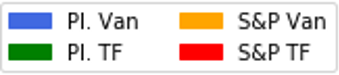
Additionally, the sentence vectors computed by TextVectors use what will be referred to in this blog as a ‘vanilla’ approach. That is, given the word vector representations, the sentence vectors are calculated as an average of the word vectors present in that sentence. These vanilla vectors perform well, but theoretically we know that certain words are more important than others, so we also implement an approach to weighting their importance in calculating sentence vectors that is commonly known as term frequency inverse document frequency (tf-idf).
Tf-idf weighting allows terms that appear multiple times in a sentence to contribute more to that sentence’s vectorized ‘meaning’, but less so if that term occurs often across all sentences in the data. This is useful for reducing the vector contribution of frequently occurring but semantically irrelevant terms, which might be obvious stop words such as ‘a’ or ‘the’. More importantly, it can also catch subject-matter specific terms not normally present on lists of common stop words but whose ubiquity in the specified corpus means they are less or not important.
Examples that come to mind in the corpus of SEC filings are the words ‘statement’(s) and ‘business’, among others. These are all examples of ‘business statements’ after all!
In the example word cloud below, we see the word ‘Matters’ is so common, it probably doesn’t matter…
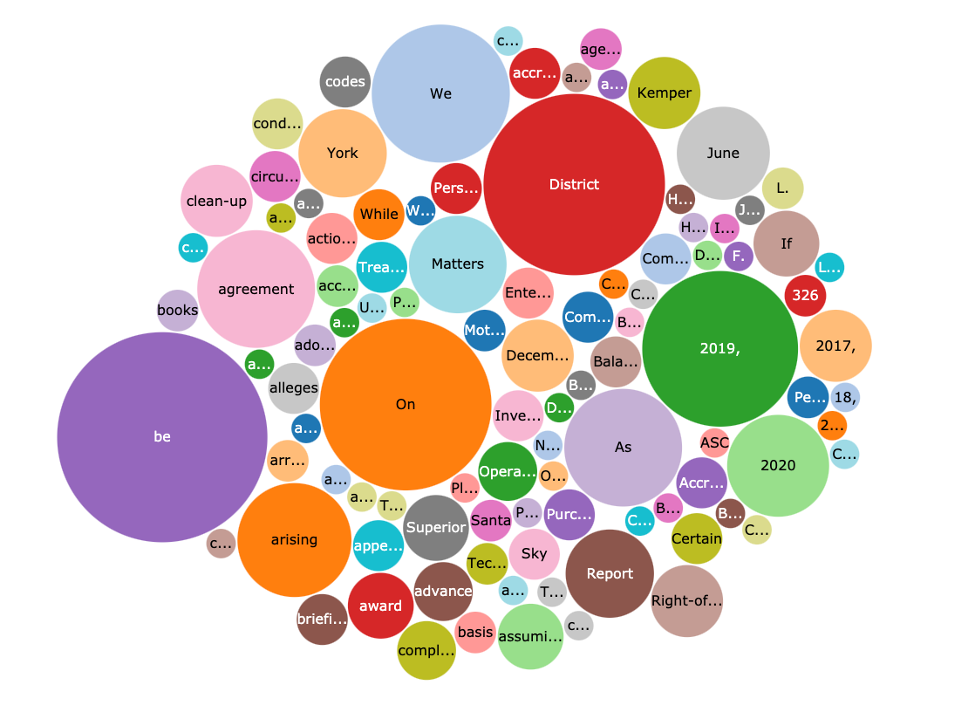
Both vanilla and tf-idf vectors are used in modeling and the relative performance of models based on each input type are compared in this project.
Dependent Variables (labels)
As previously mentioned, in this first approach to the problem, we have chosen next-quarter comparative stock performance to create binary labels for sentiment classification. That is, given a stock and the date on which its quarterly filing was submitted, if the end of the following fiscal quarter has already occurred, the closing price on the date of that end of quarter is used to calculate the label. Initially, this simple approach was used:
assign 1 if the end of next quarter is a higher stock price than on the filing date, otherwise assign 0
Students of finance will immediately see a problem with this. Individual stock performance is at least partially correlated to the performance of the overall stock market. That is, a company can report record sales, but if unrelated negative events cause investors to broadly flee risk assets (stocks, for example) that stock price could still go down.
One approach to remedy this is to compare the percent change of the stock with the percent change in the overall market. Another approach is to compare the percent change of the stock with the percent change in a basket of stocks in its industry sector, such as in an ETF covering that industry.
So far labels based on percent performance compared to the S&P 500 have been implemented and are used in our models, but the latter ETF approach may prove even more fruitful.
Modelling
Model Type(s)
There are many ECL libraries conveniently available for using machine learning models. The initial model type we used for sentiment modeling was binomial logistic regression, a form of binary classification. This can be found in the LogisticRegression bundle. Other models being considered and compared in performance are binary classification using random forests (LearningTrees bundle), support vector machines (SupportVectorMachines bundle) and others. It is also of interest to evaluate the performance of unsupervised methods such as clustering in predicting these labels.
Since the model provides us with sentence vectors and word vectors but not necessarily document vectors, two approaches to predicting document sentiment were used. The first involved assigning the document labels to each sentence from that document, training a sentiment model on the sentences, averaging the predictions from each sentence in a document, and then training a separate model on those values. The second involved creating a document vector to directly train a sentiment model on, bypassing a sentence sentiment training step. In this project the latter approach involved simple averaging of the constituent sentence vectors, but other approaches including convolution were considered for future work.
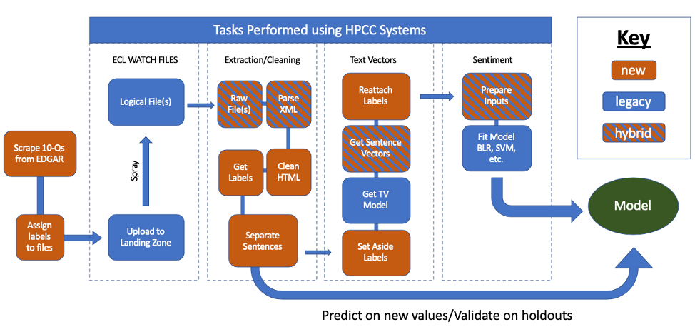 The pipeline for modeling sentiment on sentences. Document sentiment is either calculated from sentence sentiments or before labels are reattached sentence vectors are collapsed to document vectors
Parameters
There are parameters to consider at two steps: the TextVectors model used to obtain the independent variable representations, and the supervised learning model being trained on the sentiment classification task.
The parameters used for the BLR models were set to the default in the HPCC Systems Logistic Regression bundle (max_iter=200,epsilon=1E-8).
The parameters used for the CF models were fit with all parameters on default (numTrees=100, featuresPerNode=0[sqrt(# of features)], maxDepth=100, balanceClasses=FALSE), except for maxDepth, which was tested at maxDepth = 100, 50, 25, and 10 to check for under/overfitting or performance/speed differentials.
Perhaps most importantly, the underlying text model parameters were left on bundle defaults (vecLen=100[hidden layer size], trainToLoss = 0.05, numEpochs = 0[no fixed number], batchSize = 0[auto assign # of actions before syncing nodes], negSamples = 10, learningRate = .1, discardThreshold = 1E-4, minOccurs = 10, wordNGrams = 1[unigrams only], dropout = 3). The trainToLoss value was varied in initial experiments with this data but the text model’s final training loss from default parameters (0.09) was not found to vary more than 1E-3 with changes in magnitude of the loss parameter.
Future work would compare performance of bi- and tri-gram models in order to better capture the nuances in combined word phrases for this subject matter – ‘low costs’/’high costs’ could be more informative than just ‘costs’ averaged with ‘high’ or ‘low’.
Training
A function was written to separate the data into training and testing sets according to filename, stock ticker, or sentence number. Ultimately, separate models were trained separately for each industry sector, with holdout sets designated according to stock ticker in order to avoid representing the same document in the train and test set.
It’s pretty satisfying when you’ve got everything in the right format and you get to click Run and see results…but we’re not finished yet!
Tuning
Based on the initial results, it may become desirable to account for various factors and change something about the independent or dependent variables or the model parameters in order to improve results and model reliability.
For example, I found that results hardly differed between Classification Forest depths of 50 and 100, but the difference in the time to train was significant. This tradeoff also may have been preferable in regards to avoiding overfitting. On a more fundamental level, it was only after a slew of training missteps with sentence/document models that it occurred to me to directly train document vectors. Model improvement may be an ongoing process.
Testing/Validation
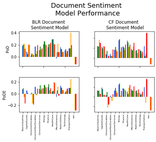
The main metrics examined on labeled holdouts were Power of Discrimination (PoD) and Power of Discrimination Extended (PoDE). The former refers to the performance of a model relative to a random (naïve) guess of class. That is, given two classes the random guess of class assigns a .5 probability, so a .6 accuracy would result in a .2 PoD. The latter refers to the performance of the model relative to the performance obtained by guessing the most prevalent class in the training set. That is, given two classes, assuming one is present in 60% of samples and the other in 40% of samples, an accuracy of .7 would get a PoDE score of .25. As a result, any model with a PoDE greater than 0 performs better than a trivial solution.
The direct document sentiment model performance vastly outperformed the document/sentence approach, with most sectors exhibiting an out-of-sample (train/test split performed on ticker symbol) PoDE of between 0.1 and 0.25.
Incidentally, a test on 14 documents from the most recent quarter without labels appeared to result in a positive return of 80% (using plain/absolute label scheme and ‘vanilla’ vectors) on choosing to invest $1,000 in each identified positive sentiment filing – 8 documents out of the 14 were identified to have positive sentiment and the sum of their percent changes was 80%. These results are tantalizing, but are unlikely to be reproducible. The recent quarterly filings tested represent too small of a dataset to concretely support this approach when risking capital, especially given the notorious difficulty in predicting stock performance. Further research is warranted, including back-testing on a larger historical dataset.
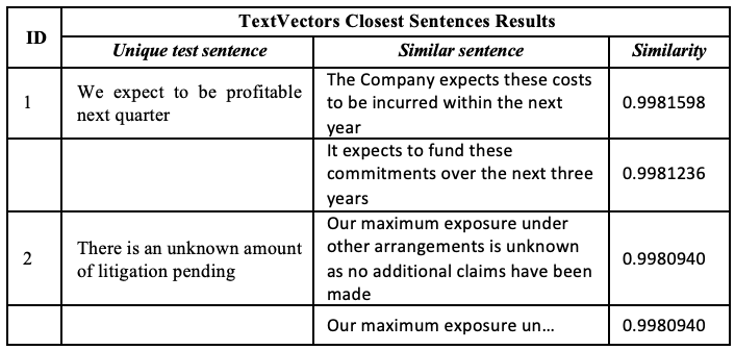
A test of closest sentence within the corpus on two new sentences I generated is shown in the below table. It is evident the model is correctly identifying the unigrams it was trained on, though it may be missing the nuances of sentiment from a basic similarity standpoint. The latter sentence result indicates the inherent redundancy in some of the data. Further work is warranted to improve the language model.
Similarity Model
The second approach, similarity, takes the vector representations of sentences generated from the TextVectors model (either vanilla or tf-idf) and uses them to compare the documents they come from.
As an example, assume Document A has three sentences:
‘The SEC has a lot of regulations. We believe that this will not have a material impact on our operations. The preceding is forward-looking information provided by the company to interested parties that may or may not be reflective of future business actions.’
Now assume Document B has two sentences:
‘After an environmental cleanup, the issues have been successfully mitigated. The preceding is forward-looking information provided by the company to interested parties that may or may not be reflective of future business actions.’
For simplicity, let us assume that the sentences that are not exactly the same in this case have a similarity of 0 (in practice, they will have a non-zero similarity because they are likely to share multiple words – how high this similarity is will depend on how many words they share, and in the case of tf-idf, how important those words are to the core meaning of that sentence). Then we have six sentence pairs:
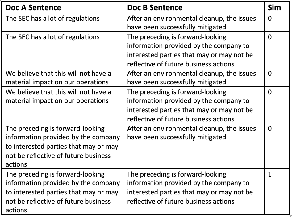
To get the doc to doc similarity, we would then take the average of these sentence similarities: there is only one shared sentence between them, so since for simplicity we are calling similarities between sentences that are not exactly the same 0, the overall score here is 1/6, or .16666. Again, in practice, the sentences share many words, so the 0 scores are more likely to be in the range of .8 or .9, and our final score would be much higher. However, our process is the same: take the cosine similarities of sentence pairs and take the average of those values to find the overall document similarity.
This averaging approach allows for recognition if there are entire sections that are the same between two documents, but keeps the score from being overly high if that section accounts for a small part of one document. Another approach that was found to be more strongly influenced by lower similarity values (and therefore ultimately more informative), involved taking the nth root of the product of sentence pair similarities (with n the total number of sentence pairs).
So far, this analytic approach to the text vectors is being examined by calculating similarity for successive quarterly filings and comparing this to their sentiment labels to determine correlation or predictive value.
These tools are only a few examples of what is possible with TextVectors and HPCC Systems on such a problem. As previously mentioned, the cleaned data is useful even when packaged for simple data query, perhaps by securities analysts or financial advisors. This is already possible. Given a logical file path, simply read in with the EDGAR_Extract module and query the fields of interest. A more streamlined function may be rolled out, but to reiterate the original point, our work unlocks more value through interdisciplinary efforts. That is to say, there are plenty of interesting directions that development could go next, for example, using a different NLP architecture such as attention-based transformers, remodeling sentiment based on legal data on regulatory filings against banks (rather than stock performance) in order to find filing language associated with adverse outcomes, and quite a bit more.
More about this project and Matthias’s contribution to our open source project
During Matthias’s internship he was mentored by our LexisNexis Colleagues, Lili Xu (Software Engineer III) and Arjuna Chala (Senior Director Operations) and was also supported by Roger Dev (Senior Architect) who is the leader of our Machine Learning Library project.
Matthias’s project covered a lot of ground and he achieved a lot during that time but his contribution to our open source project does not stop at the end of his internship. He has checked in his code and supporting documentation which will be made available to our open source community in the coming months. His work is a valuable addition to our Machine Learning Library and will be wrapped up into a bundle making it easy to access and use.
References
- [1] Cohen, Lauren et al. “Lazy Prices” The Journal of Finance. Vol. 75. Issue 3. 2020
- HPCC Systems TextVectors bundle, supporting documentation and tutorial.