Introduction to using PBblas on HPCC Systems
One of the main pieces of preliminary work involved in the major refactoring of the HPCC Systems Machine Learning Library was to productize PBblas as the backbone for Matrix Operations. The Parallel-Block Basic Linear Algebra Subsystem (PBblas) provides a mechanism for adapting matrix operations to Big Data and parallel processing on HPCC Systems clusters.
PBblas allows matrix operations of nearly any scale to be effectively computed on HPCC Systems. Let’s have a look at the capabilities and approaches inherent in PBblas.
- Matrix representation
- Automatic partitioning and workload balancing
- Myriad capabilities
- Some Usage Examples
- Installing PBblas
- PBblas performance
Matrix Representation
PBblas matrices are stored as a DATASET(Layout_Cell). See PBblas.Types.Layout_Cell. Each record in the dataset represents one cell in a matrix. Layout_Cell has the following fields:
- wi_id – The work-item-id. Many separate matrices can be included in a single dataset, each assigned a separate wi_id.
- x – The row number of this cell in its matrix
- y – The column number of this cell in its matrix
- v – The numerical value of the cell
Layout_Cell is a sparse matrix format. That is, only non-zero cells need to be supplied. Any cells that are not in the dataset are assumed to be zero. All external interfaces to PBblas utilize this format. Internally, PBblas may utilize dense or sparse matrix storage.
Most HPCC Systems machine learning algorithms use NumericField and DiscreteField to hold matrices (a topic for a future blog). PBblas provides a “Converted” module that provides attributes to convert between these formats and Layout_Cell.
Automatic Partitioning and workload balancing
Internally, matrices are automatically split into bite-sized pieces called “partitions”. The size and shape of PBblas partitions are automatically determined by an algorithm that takes into account several factors:
- The sizes of the matrices
- The number of nodes in the cluster
- The operations being performed on the matrices
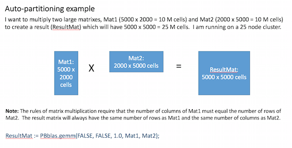
Based on these factors, an appropriate partitioning scheme is chosen for each matrix. The example below illustrates how this works for a matrix-multiplication operation:
Internally, Pbblas determines an effective partitioning scheme such that:
- The partition scheme for the largest matrix is square (i.e. N x N partions), row-vector (i.e. N x 1) or column-vector (i.e. 1 x N).
- Partition scheme obeys the rules of matrix multiplication (i.e. # of Mat1 column partitions = # of Mat2 row partitions AND # of Result row partitions = # of Mat1 row partitons AND # of Result column partitions = # of Mat2 column partitions.
- Each partition obeys the rules of matrix multiplication (i.e. # columns of each Mat1 partition = # rows of each Mat2 partition AND # rows of each result partition = # rows of each Mat1 partition AND # columns of each result partition = # columns of each Mat2 partition).
- No partition is > Max_Partition_Size (default 1 M cells) in order to avoid memory exhaustion.
- The number of result partitions is an even multiple of the number of nodes in the cluster (to balance the workload).
- Partitions are as large as possible, subject to the above constraints (in order to maximize performance of matrix operations on each node, while minimizing distribution costs).
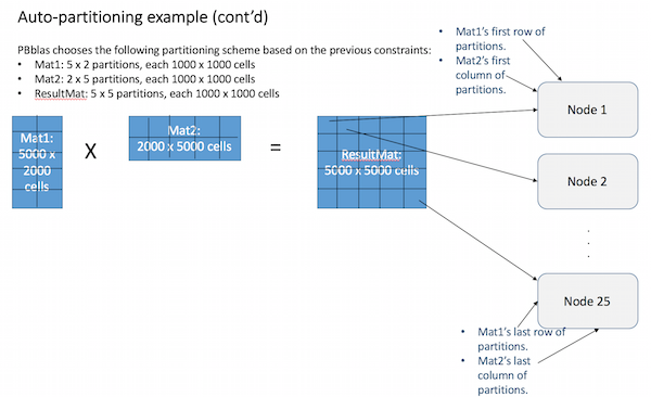
PBblas will now treat the partitions as if they are cells in a much smaller matrix, following the same rules of matrix multiplication:
- First, the result partitions are each assigned to a cluster node.
- Then the partitions of Mat1 and Mat2 that are needed to compute each result partition are copied to the corresponding nodes.
- The partitions are multiplied locally on each node as if they are individual cells.
- The cells in each partition are multiplied locally using the C BLAS library.
- This results in a full solution that is now distributed across the cluster.
- Each node only had to solve 1 result partition, so the workload was balanced.
- This illustrates the process with a convenient set of matrix and cluster sizes. In practice, partition sizes are not likely to be the maximum (1M) and nodes may each have many partitions to process. Each node will almost always be assigned an equal number of partitions, however.
A similar partitioning approach is used for other PBblas operations such as matrix factoring and solving (discussed later). Keep in mind that partitioning addresses several scaling issues :
- Parallelizing the process so that we can take advantage of all the nodes in a cluster.
- Reducing an operation that normally needs to be memory-resident into a series of smaller operations that can be handled sequentially on a node without exhausting its memory.
It is interesting to note that some of the partitioning approaches utilized by PBblas were originally developed in the 1950’s and 1960’s, when computer memory was too small to execute operations on even modest sized matrices. We now use these same techniques to scale today’s systems to handle modern Big Data requirements.
Myriad Capability
All of our new machine learning bundles provide a capability known as “Myriad”. This allows a given operation to execute on many matrices at a time, as illustrated below:
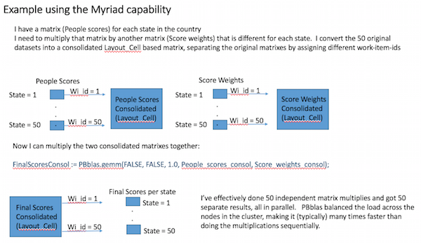
By combining many matrix operations into one operation, we can better utilize the parallel processing power of an HPCC Systems cluster, even when each matrix operation may only be large enough to require one or two nodes.
PBblas Operations
The PBblas interface is modelled on the time-tested and defacto standard interface for matrix operations known as the Basic Linear Algebra Subsystem (BLAS), which has been in use for many years. The authors of BLAS recognized that Linear Algebra operations are not typically used in isolation, but in sequences of operations to perform tasks such as machine learning. They also recognized that when common sequences of operations are done in a single step, some of the operations can be had for free, or at least with far less compute time than if done one at a time.
For this reason, most of the BLAS (and therefore PBblas) operations provide a compound series of simpler operations that are commonly used together, and that are more efficient than doing the simpler operations sequentially. Let’s look at the PBblas function “gemm” for example. While the central purpose of gemm is to multiply two matrices, A and B, its full definition is: alpha * A(T?) * B(T?) + beta * C. Note that the (T?) indicates that the matrix is to be transposed (turned on its side) before the multiply. So in its fullest form, gemm will transpose matrix A, scale it by factor “alpha”, transpose matrix B, multiply the two modified matrices together and then add it to another matrix C after it has been scaled by “beta”. This can all be done at very close to the same cost as a basic matrix multiply.
The PBblas operations include:
- Gemm – Multiply two matrixes, with optional scaling and transpose. Add an optional third matrix (with optional scaling) to the resulting multiplicand.
- Axpy – Optionally scale a first matrix and add it to a second matrix.
- Getrf – Factor a matrix into Upper and Lower triangular matrixes.
- Potrf – Factor a matrix using Cholesky factorization to produce a matrix that, when multiplied by its transpose will produce the original matrix (analogous to the square-root of a matrix).
- Scal – Scale a matrix by a constant.
- Tran – Transpose a matrix and optionally add it to a second matrix with optional scaling of the second matrix.
- Trsm – Solve a triangular matrix operation of the form AX = B or XA = B (solving for X). Includes optional scaling or transposing of the A matrix.
- HadamardProduct – An element-wise multiplication of two matrixes.
- Asum – Sum the absolute values of cells of a matrix to produce the “Entrywise 1-norm”.
- ApplyToElements – Apply a user-provided function to each cell of a matrix.
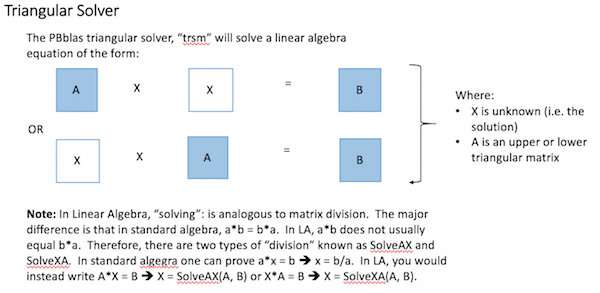
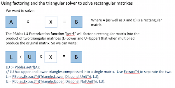
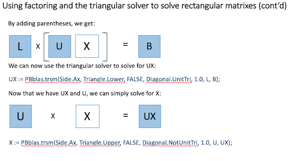
Matrix Solving
PBblas provides a triangular solver, which requires that the A matrix is an upper or lower triangular matrix (i.e. with all zeros below or above the diagonal respectively). It uses a triangular solver because there isn’t an efficient algorithm for directly solving rectangular matrixes in a distributed environment.
Using basic Linear Algebra, a rectangular matrix equation can be solved by factoring the square matrix into two triangular matrixes and then properly applying the triangular solver, as shown here:
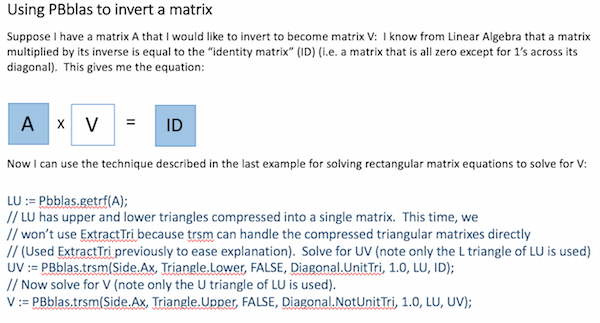
Matrix Inversion
It is sometimes useful to invert a matrix. It may not be obvious how to do this, given the operations described above. This example shows how it can easily be achieved using PBblas operations and a bit of Linear Algebra:
Installing PBblas on your system
PBblas is packaged as an HPCC Systems bundle, which can be installed independently of the Platform. PBblas requires HPCC Systems platform versions 6.2.0 as a minimum. All platform versions since 6.2.0 (download the latest here) automatically include the BLAS library, which is a prerequisite for using PBblas. The PBblas bundle is also dependent on the HPCC Systems Machine Learning Core Bundle (ML_Core).
- Make sure HPCC Systems Client Tools package is installed for the operating system you are using.
- Download the ML_Core bundle from GitHub.
- Download the PBblas bundle from GitHub.
- Using HPCC Systems Client Tools, install the two bundles in order from the clienttools/bin folder:
-
ecl install bundle <path to ML_Core bundle> -
ecl install bundle <path to PBblas bundle>
-
- Run the Multiply.ecl test (PBblas.Test.Multiply) and verify that it completes with no errors
- Optionally run other tests such as PBblas.Test.Solve.
- Then write some ECL to perform matrix operations!
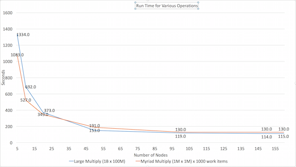
Performance characteristics
The Large Multiply multiplies a 1B cell matrix (100K rows by 10K columns) by a 100M cell matrix (10K rows by 10K columns).
The Myriad Multiply test does 1000 small matrix multiplies of 1M cells (1000 x 1000) by 1M cells (1000 x 1000) in a single operation.
Here are the results of our own testing:

Hardware configuration details
AWS Server type R3.8xlarge
5 servers, 32 virtual CPUs each
Changed “slavesPerNode” to achieve the desired “node-counts”.