Causality 2021

Causality 2021 is an HPCC Systems research and development program designed to understand the latest developments in Causal Sciences, evaluate the effectiveness and limitations of the current state-of-the-art,  push the boundaries of causal inferencing, and develop a full-bodied Causality Toolkit for HPCC Systems.

What do we mean by Causality?

Causality as a science is fairly new, and is evolving rapidly.  Though people have been discussing causality for thousands of years, it was resigned to philosophical discussion. It had little scientific underpinning until the past 30 years, and did not have a cohesive mathematical basis until Pearl’s seminal work in 2000 [1] for which he won the prestigious Turing Award.

Causality is a natural layer of knowledge and practice, layered on Statistics, as Chemistry is layered on Physics, and Biology is layered on Chemistry.  In practice, Causality provides two distinct layers on top of traditional Pearson / Fisher statistics.  Pearl [2] characterizes this relationship as the Ladder of Causality as depicted below.  The Ladder has three rungs:  Seeing (statistics), Doing (intervention), and Imagining (counterfactuals).

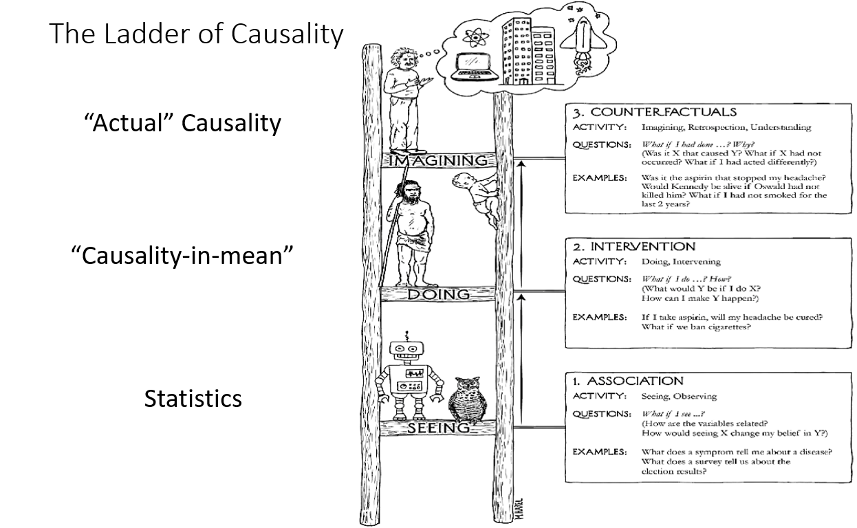
Statistics is about observing patterns in data, or “seeing”.  The Joint Probability Space of a multivariate (i.e. multiple variable) dataset encodes everything knowable about the data — the behavior of each variable individually, and the relationships between variables.  But when it comes to cause and effect relationships, statistics can say little, except in highly controlled settings.  Fisher correctly contended that the only way to understand cause and effect through statistics is via randomized, controlled experiments.

Intervention is about “doing” — observing what happens when changes are made to the causal structure underlying the data.  This can be characterized as causal exploration.  What would happen to Y if we tweaked X and Z?  It is the layer of what-ifs.  There is a price of admission to this layer, however.  And this admission price is what forms a clean boundary between the first two rungs.  While Statistics only requires data, Intervention requires data plus a model of the underlying causal structures that produced the data.  Armed with these two prerequisites, one can perform computations that are impossible to even specify within the realm of Statistics.  We can perform calculations such as: what would have been the value of Y if we set X to .5?  At first glance, this may sound like a statistical question, but the closest we can ask statistically is: what does Y look like when we see X at a value of .5?  The distinction is very important — seeing vs doing.  I’ll attempt to illustrate this further below, but first let’s look up over the second rung to the third rung.

Counterfactuals can be thought of as “imaginings”.  This is a world not available at Rung 2 of the Ladder.  It allows us to consider specific scenarios that are unthinkable and inexpressible at Layer 1 or 2.  What would have happened to Bob if he hadn’t had the treatment, given that he did and recovered?  Would the accident have occurred if the traffic light had not been broken?  Counterfactuals are in play whenever there is a could, would, or should in a question.  But many questions that appear straight-forward on the surface, and don’t contain those conditional words, actually translate to counterfactuals as well.  Questions like: What caused the accident?, or “Did the treatment kill Charlotte?”.  The latter can be translated to the counterfactual:  “What is the probability that Charlotte would have died had she not gotten the treatment?”.

Correlation always implies Causality

We learn from day one in introductory Statistics that : “Correlation does not imply Causality”.  While this is true in the sense it was intended, it leaves us with two uncomfortable questions:  What does correlation imply?, and “What does imply causality”.  The new science of Causality provides clear and useful answers to both these questions.  My tongue-in-cheek heading above is also (nearly) true.  With very rare exceptions, correlation is the trace effect of causal relationships.  Causality creates correlation, but not necessarily in a straight forward way, so read my heading as “Correlation Always implies that there are causal relationships between data elements”.  If A and B are correlated, it may not be the case that A causes B or that B causes A.  It may be that C has an effect on both A and B.  But in any case, you can be confident that A and B have a direct or indirect causal relationship.  Causal algorithms can often tease apart these relationships and uncover the mechanisms that produced the data.  Once these have been identified, then whole new worlds of computation open up.  An adequately understood causal model allows causal inference from purely observational data.  I’ll use an absurd scenario to illustrate how this works in practice:

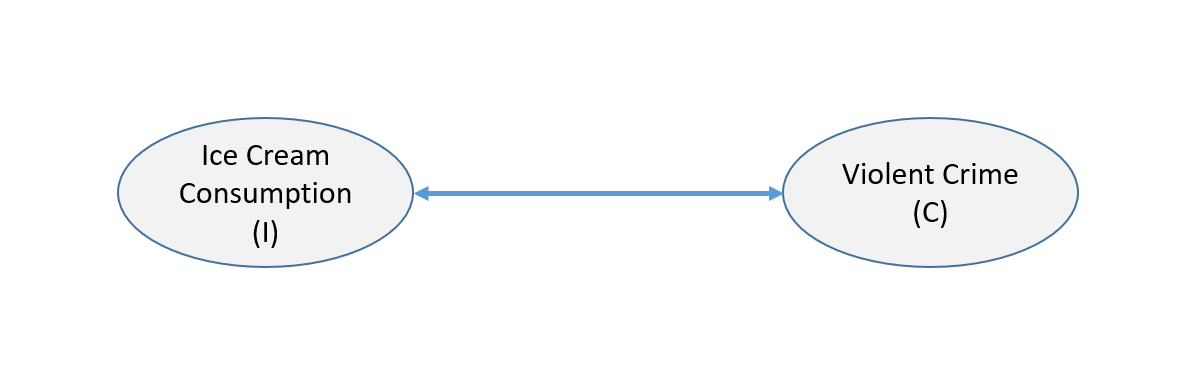
It’s been observed that Ice Cream consumption in Chicago is correlated with Violent crime.  Presented with such a scenario, our first inclination is to think that it must be a coincidence.  It doesn’t make sense.  Our mind rebels.  We inherently believe that correlation means something causal, but what does the correlation mean?

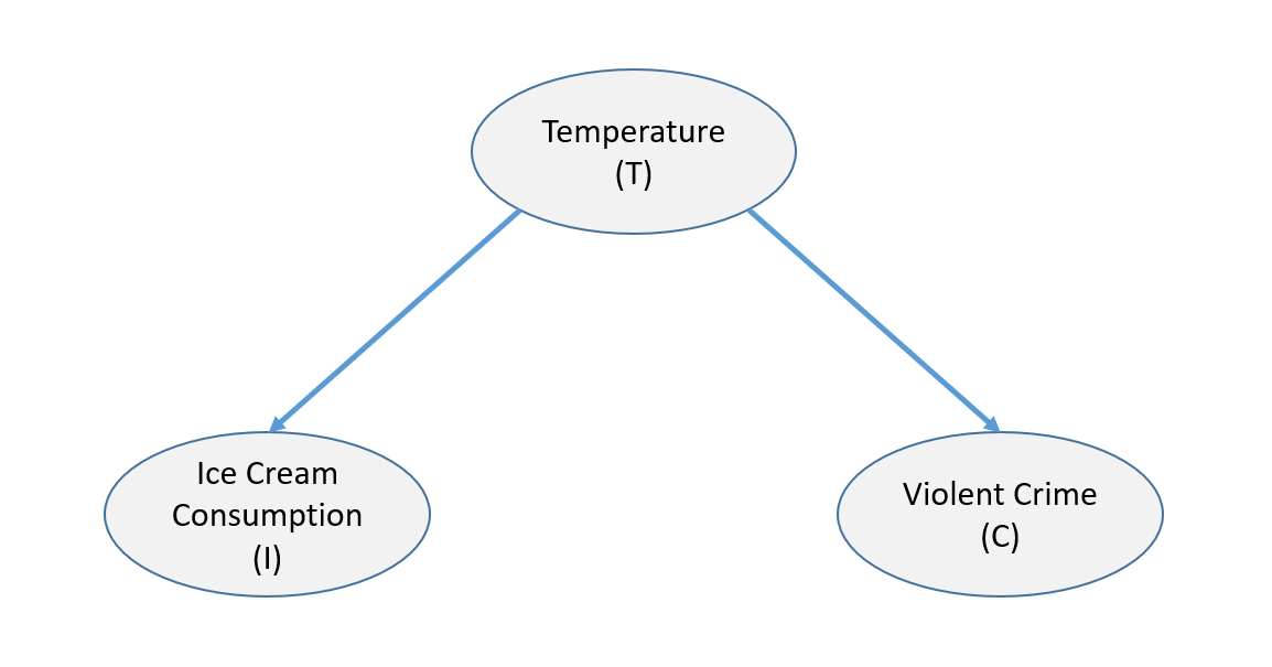
If I even mention a third variable: Temperature, your mind has probably already jumped to the correct causal model:  Temperature affects both Ice Cream consumption and Crime.

Okay, that makes sense. But is it possible that Ice Cream and Crime are also related through some other mechanism?  We could conduct a controlled experiment, forcing random people to either consume ice cream or not, but that would be costly and unpopular.

Armed with this causal model, and data on crime, ice cream consumption and temperature, we can ask questions like:  Does Ice Cream have any effect on Crime?  How strong an effect?  The Causal Calculus tells us exactly how the answer is computed.  The path to its solution provides insight into the nature of intervention:

Note that all three variables are correlated.  It is useful to think of correlation following the causal arrow lines, but ignoring  the direction of the arrows.  Correlation flows between Ice Cream and Crime through Temperature, while Causality has a definite direction — from the cause to the effect.  Therefore, if we could block the correlation from flowing through temperature, then any remaining correlation would have to be directly from ice cream to crime, or crime to ice cream (barring a fourth variable).  Fortunately there is a mechanism that can block this correlation.  It is our old statistical friend “conditioning”.  If I take a small temperature range (e.g. 2 degrees), and observe the correlation between ice cream and crime for days that have temperatures in that range, we should see no correlation related to temperature.  If I condition on every such small temperature range, and average them together, I should then see no correlation for any given temperature range, and therefore no correlation in the total.  So if I look at the correlation between ice cream and crime given temperature (i.e. Correlation(ice cream, crime | temperature)), I would expect to get zero, even though ice cream and crime are correlated.  We can say that conditioning on a variable “blocks” the flow of correlation through that variable.  Now if I found any correlation, I would want to measure its strength by “intervening” on ice cream.  I could set ice cream consumption to a low level, and observe its effect on crime, I could then set ice cream consumption to a high level, and see how much crime increased.  I could calibrate the results as the average effect of ice cream on crime (i.e. ACE(ice cream, crime).   And I can run the experiment analytically, without ever telling anyone whether to eat ice cream or not.

Scope of causality

There are a number of different functional areas comprising Causality

• Model representation
• Model discovery
• Model validation
• Interventional Inference
• Counterfactual Inference

Underlying these areas, are a set of statistical techniques that are required in order to process the causal algorithms.  These techniques, while within the realm of Rung 1 — Statistics, are heavily used within a Causal context and require high degrees of performance and accuracy in order for Causal computations to be practical.  These include:

• Conditional Independence Testing
• Conditional Probability
• Directionality Testing

Project Progress and Status

We set out to implement all of the different functional areas in a way that provides minimum constraints on the data being analyzed.  We therefore decided that we needed to handle both discrete and continuous variables, and make no assumptions as to the relationships among them.  This implies that we cannot rely on any mathematical crutches such as linearity or parametric distributions.  We decided to focus on what’s known as “contemporaneous causality” first, and defer time-series causality, which has its own sets of algorithms.

Synthetic Data Generation

In order to test our various algorithms, we need to be able to generate rich multivariate datasets with known characteristics so that we can know if our answers are correct.  We developed a Structural Equation Model (SEM) based synthetic data generator that allows us to generate such datasets.  We think this will be useful, not only for testing Causal algorithms, but for many other analytic methods in the future.

Statistical Layer — Rung 1 — “Seeing”

At the base of the system is a statistical analysis system: ProbSpace that allows us to extensively query the  joint probability space of a multivariate data set.  Recall that the joint probability space encompasses everything knowable from the data.  That means that not only does it support a wide range of queries about probabilities, joint probabilities, and conditional probabilities, but also can calculate correlation, independence, directionality, and prediction.   Note that the types of questions answered by machine learning are also answerable by a simple query of the joint probability space.  The classical machine learning question is: What is the most likely value of Y given X1 = val1, X2 = val2, etc. That is a basic conditional probability question, easily answered for any variables within the joint probability space.

Our original, somewhat naive approach was to discretize the continuous variables so that we could treat everything uniformly as discrete variables, albeit with very many discrete values.  We call this approach “Pre-Discretization”.  This proved to be too confining, and we evolved to separate algorithms for discreet and continuous data.  In this approach, discretization is done during the query, which allows queries to intelligently discretize results on the fly.  We characterize this as “Post-Discretization.  This produced very good results in most cases, but suffers from a number of drawbacks: First, the tails of each distribution have very few data points, and the observed distribution may not correspond very well, therefore, to the generating distribution.  Second, conditioning on multiple variables encounters the so called “curse of dimensionality”, requiring exponentially more data as the conditioning set becomes larger.  This limits the types of queries that can be accurately answered.

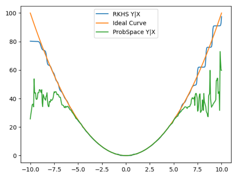
These issues affect two aspects of the probability system:  Conditional Probabilities, and Conditional Independence Testing.  Our research indicated that the best state-of-the-art methods utilized Replicating Kernel Hilbert Spaces (RKHS) for both aspects.  Understanding these spaces has been challenging, but has shown very good preliminary results.  The graph below, shows the Expected value of Y given X, where Y is a non-linear function of X (in this case Y = X squared plus noise).  The green line shows the results for the post-discretization method.  Notice that the results are almost perfect until we get to the far tails of the distribution, where they break down rather dramatically due to the very few data points available.  The blue line shows the RKHS solution, which is near perfect in the rich parts of the distribution, and still very closely follows the curve as we get into the tails.

Here is a link to a Mini-Primer on RKHS for those interested in learning more about this useful technique.

Intervention Layer — Rung 2 —  “Doing”

This layer allows queries that are not expressible statistically.  Specifically, it includes a “do()” operator.  This supports “what-if” types of queries such as:  What would the distribution of A be if we set B to .5 and C to -3 (i.e. P(A | do(B=.5, C=-3))?.  This is analogous to conducting a controlled experiment, where B and C were held at particular values.  It does this by symbolically severing the causal links between B and its parents (causes), and A with its parents, to force them to take on particular values.  Based on the resulting altered causal model, the causal and non-causal components influencing A are separated, and the result of the intervention is computed.  This layer provides all of the queries available at Rung 1, with the addition of intervention capabilities.  Interventions deal with aggregate effects of setting variables to fixed values.  It is sometimes referred to as “Causality-in-mean”.  It cannot answer questions about individual results.

We currently have a working prototype of this layer.  It is able to process Interventions, as well as calculate certain causal metrics such as Average Causal Effect (ACE), and Controlled Direct Effect (CDE).

Counterfactual Layer — Rung 3 — “Imagining”

We are just beginning to implement this layer.  It will allow any Rung 1 or Rung 2 queries, plus Counterfactual queries.  Counterfactual queries take the form “What is the probability that <some set of things are true> in the closest alternate world where <some condition> is true given that <some condition> was false and we observed or did <some other things>”?  This can be used to answer should, could, or would questions, as well as some unobvious counterfactuals like: “What caused the outage?”, “Did the treatment save Carl?”, or “What is the best dose of medicine for Sally?”.  Counterfactuals deal with specific observations, which might be people, vehicles, trees, or any other type of entity represented by a given dataset.

Model Validation, Causal Discovery, and Causal Scanning

Nature has left us with some very subtle signals within data to indicate the causal relationships that generated that data.  These signals can be hard to detect, and prone to statistical error.  Yet the human mind seems to have an uncanny ability to reason about causes.  In the Ice Cream / Crime scenario above, as soon as temperature was mentioned, you were able to quickly determine that Temperature causing Ice Cream consumption and Crime was a much more likely model than Crime causing Ice Cream consumption, or Ice Cream consumption causing crime.  Our minds are extremely nimble with this ability.  Given any scenario with which you are even vaguely familiar, you can propose a sensible causal scenario, or perhaps a few possible scenarios.

In an ideal scenario, we will know the causal model, and will be able to then directly draw Interventional or Counterfactual inferences using those query layers.  It is likely, however, that there may be aspects of the model where we are not certain.

The Causal Model, as depicted in Figure 3 above, describes the process that generated the data.  When we know both the data and the generating process, we can infer interesting things that cannot be computed from the data alone.  Arrows go from cause to effect, and are best read as “has an effect on”.  A Directed Acyclic Graph (DAG) is used to represent the model.  This just means that the lines (with their arrows) imply direction, and that there can be no cycles in the graph such as A->B->C->A.

Each causal model, in fact, represents a hypothesis of the true causal relationships (i.e. generating process).  We can use Model Validation to test whether our data matches the hypothesized model, or which of several models  best fits the data.

We have developed a Model Validation test that compares the data with the model, and outputs a set of errors or warnings where the data doesn’t seem to fit the model.  It then heuristically rates the fit, giving an overall confidence level. Models that score highly are probably well suited to Intervention and Counterfactual queries.

Much work has been done in the area of Causal Discovery, but this is difficult for a number of reasons:  The trace signals are typically weak, and difficult to detect, and these signals fade at each causal transition.

In some cases, we are given a dataset without an obvious causal hypothesis and we need to try and understand the model analytically.  Two techniques are used for this:

Causal Discovery includes various methods that attempt to map the causal model using the subtle trace signals in the data.  This tends to be impractical with complex datasets, due to the subtlety of the signals, and the fact that they decay with the depth of the causal tree.  The accuracy of the resulting model is hard to assess if the data is abstract enough, and use of these models as a basis for inference may not be practical.  It may however, shed insight as to the nature of the data, or provide a basis for a model that is then to be tested against common sense.

Causal Scanning is a special type of Causal Discovery.  It works hierarchically to find sets of related variables, and subsets within those sets.  It then explores the relationships between those sets at each level.  As it works its way down to the bottom-most layer, it finds relationships between smaller and smaller sets until at the bottom layer it is equivalent to Causal Discovery.  The goal of Causal Scanning is to highlight the large-scale causal relationships, even when unable to determine the exact model.

We have created a basic Causal Scanning system, and are in the process of refining it.

The Team

Our team is made up of myself and three interns:

• Achinthya Sreedar — RVCE, India — Probabilities and Conditional Probabilities
• Mara Hubelbank — Northeastern University, Boston — Counterfactual and Interventional Layers
• Mayank Agarwal — RVCE, India — Independence, Conditional Independence, and Directionality

Additionally, Lili Xu, from our Machine Learning team is assisting us on a part-time basis.

Each of the interns maintains a Blog, charting their daily progress and accomplishments.  This project involves a lot of advanced mathematics, and has been very challenging. But the interns continue to plow through it and make progress. The step by step progress reported in their blogs is inspiring and illuminating.  The Blogs are available below:

• Achinthya — https://myhpccintern.blogspot.com/
• Mara — https://marahubhpcc.blogspot.com/
• Mayank — https://mayank-causality-hpcc.blogspot.com/

Next Steps

Our project has now reached its (approximate) midpoint, and while a lot of progress has been made, much more remains to be done.  Our current focus is on optimizing the key algorithms (Conditional Probability and Conditional Independence Testing) and finishing Counterfactuals and Causal Scanning.  But two significant efforts remain:

HPCC Systems Causality Toolkit

Our current implementations are done as a set of standalone Python modules. We will then wrap these modules within an ECL interface using ECL’s Python embedding.  We understand how to parallelize most of the algorithms, and will include that capability as we design the interface.  Causality algorithms are expensive, since they are performing very deep computations on the data.  This makes the HPCC Systems Platform a natural environment for doing Causality research and application, since the algorithms parallelize nicely, and will provide much faster results.

Live Data Testing

We hope to be able to demonstrate useful results, for each of the algorithms, against real-world datasets.  Once the algorithms are complete and available within HPCC Systems, we will work on locating appropriate datasets and utilizing Causality to enhance our understanding of the data.

References:

General Causality:

[1] Pearl, Judea (2000, 2008) “Causality: Models, Reasoning, and Inference”, Cambridge University Press

[2] Pearl, Judea; Mackenzie, Data (2020) “The Book of Why: The new Science of Cause and Effect”, Basic Books

[3] Pearl, Judea; Glymour, Madelyn; Jewell, Nicholas P. (2016) “Causal Inference in Statistics”, Wiley

[4] Rosenbaum, Paul R. (2017) “Observation and Experiment:  An Introduction to Causal Inference”, Harvard University Press.

[5] Halpern, Joseph Y. (2016) “Actual Causality”, MIT Press.

Conditional Independence Testing:

[6] Li, Chun; Fan, Xiaodan (2019) “On nonparametric conditional independence tests for continuous variables” , Computational Statistics, Wiley.  URL: https://onlinelibrary.wiley.com/doi/full/10.1002/wics.1489

[7] Strobl, Eric V.; Visweswaran, Shyam (2017) “Approximate Kernel-based Conditional Independence Tests for Fast Non-Parametric Causal Discovery”,  URL: https://arxiv.org/pdf/1702.03877.pdf

[8] Zhang, K.; Peters, J.; Janzing, D.; Scholkopf, B. (2011) “Kernel-based conditional independence test and application to causal discovery”, Uncertainty in Artificial Intelligence, p 804-813.  AUAI Press.

[9] Fukumizu, K.; Gretton, A.; Sun, X.; Scholkopf, B. (2008) “Kernel measures of conditional dependence”, Advances in Neural Information Processing Systems, p 489-496, URL: https://papers.nips.cc/paper/2007/file/3a0772443a0739141292a5429b952fe6-Paper.pdf

Directionality:

[10] Hyvarinen, Aapo; Smith, Stephen M. (2013) “Pairwise Likelihood Ratios for Estimation of Non-Gaussian Structural Equation Models.”, Journal of Machine Learning Research 14, p 111-152.

[11] Shimizu, Shohei (?) “LiNGAM: Non-Gaussian methods for estimating causal structures”, The Institute of Scientific and Industrial Research, Osaka University, URL: http://www.ar.sanken.osaka-u.ac.jp/~sshimizu/papers/Shimizu13BHMK.pdf

Conditional Probability:

[12]  Hansen, Bruce E. (2004) “Nonparametric Conditional Density Estimation”, University of Wisconsin Department of Economics

[13] Song, Le; Huang, Jonathan; Smola, Alex; Fukumizu, Kenji (2009) “Hilbert Space Embeddings of Conditional Distributions with Applications to Dynamical Systems”, Proceedings of the 26th International Conference on Machine Learning, Montreal Canada, URL: https://geometry.stanford.edu/papers/shsf-hsecdads-08/shsf-hsecdads-08.pdf.

[14] Holmes, Michael P.; Gray, Alexander G.; Isbell, Charles Lee Jr. (2007) “Fast nonparameteric conditional density estimation”, URL: https://arxiv.org/ftp/arxiv/papers/1206/1206.5278.pdf

[15] Muandet, K.; Fukumizu, K.; Sriperumbudur, B.; Scholkopf, B (2017) ” Kernel Mean Embedding of Distributions:  A Review and Beyond.”, Foundations and Trends in Machine Learning: Vol. 10: No. 1-2, pp 1-141 (2017), URL: https://arxiv.org/abs/1605.09522

Causal Discovery:

[16] Glymour, Clark; Zhang, Kun; Spirtes, Peter (2019) “Review of causal discovery methods based on graphical models”, Frontiers in Genetics; Statistical Genetics and Methodology,  URL: https://www.frontiersin.org/articles/10.3389/fgene.2019.00524/full

Time Series Causality:

[17] Hyvarinen, A.; Zhang, K.; Shimizu, S.; Hoyer P. (2010) “Estimation of a structural vector auto-regression model using non-gaussianity”, Journal of Machine Learning Research 11.

[18] Duchesne, Pierre; Roy, Roch (2003) “Robust tests for independence of two time series”, Statistica Sinica 13, p 827-852.

[19] Palachy, Shay (2019) “Inferring causality in time series data: A concise review of the major approaches.”, Towards Data Science, URL: https://towardsdatascience.com/inferring-causality-in-time-series-data-b8b75fe52c46

Interventional and Counterfactual Inference:

[20] Hopkins, Mark; Pearl, Judea (2005) “Causality and Counterfactuals in the Situation Calculus”, Oxford University Press. URL: https://ftp.cs.ucla.edu/pub/stat_ser/r301-final.pdf

[21] Avin, Chen; Shpitser, Ilya; Pearl, Judea (2005) “Identifiability of Path-Specific Effects”, Proceedings of International Joint Conference on Artificial Intelligence. URL: https://ftp.cs.ucla.edu/pub/stat_ser/r321-ijcai05.pdf

[22] Malinsky, Daniel; Shipster, Ilya; Richardson, Thomas (2019) “A Potential Outcomes Calculus for Identifying Conditional Path-Specific Effects”, Proceedings of the Twenty-Second International Conference on Artificial Intelligence and Statistics. URL: https://arxiv.org/pdf/1903.03662.pdf

[23] Pearl, Judea (2001) “Direct and Indirect Effects”, Proceedings of the Seventeenth Conference on Uncertainty in Artificial Intelligence. URL: https://ftp.cs.ucla.edu/pub/stat_ser/R273-U.pdf

Application:

[24] Xu, Xiaojie (2017) “Contemporaneous causal orderings of US corn cash prices through directed acyclic graphs”, Empir Econ 52: p 731-758.