ECL Tip – Leveraging the Power of HPCC Systems? Use AGGREGATE.

This ECL Tip spotlights the Enterprise Control Language (ECL) AGGREGATE built-in function. ECL AGGREGATE has been seen by many in the community as ‘complex,’ and as such, has been underused. However, in using AGGREGATE you can be sure you’re playing to the strengths of HPCC Systems.

Allan Wrobel, a Consulting Software Engineer at LexisNexis Risk Solutions, spotlighted the ECL AGGREGATE function during HPCC Systems Tech Talk 23, as part of the monthly “ECL Tips.” Allan is a contributor to our Tech Talks, and provides valuable information on programming with Enterprise Control Language (ECL).

In this blog, we:

• Discuss the ECL AGGREGATE  built-in function
• Provide examples of various ways to summarize data.

Let’s begin by defining ECL AGGREGATE and explaining how it works.

AGGREGATE

The ECL AGGREGATE function is used to summarize data in a dataset and present results in the form of tables. This allows for easier analysis of large amounts of data. The AGGREGATE function is similar to ROLLUP, except its output format does not need to match the input format. It also has similarity to TABLE, in that the groupingfields (if present) determine the matching records, such that you will get one result for each unique value of the groupingfields. The input recordset does not need to have been sorted by the groupingfields.

AGGREGATE (recordset, resultrec, maintransform [, mergetransform (RIGHT1, RIGHT2)] [, groupingfields]

Recordset – The set of records to process.

Resultrec – The RECORD structure of the result record set.

maintransform – The TRANSFORM function to call for each matching pair of records in the recordset. This is implicitly a local operation on each node.

mergetransform – Optional. The TRANSFORM function to call to globally merge the result records from the maintransform. If omitted, the compiler will attempt to deduce the merge from the maintransform.

groupingfields – Optional. A comma-delimited list of fields in the recordset to group by. Each field must be prefaced with the keyword LEFT. If omitted, then all records match.

How AGGREGATE Works

In the maintransform, LEFT refers to the next input record and RIGHT the result of the previous TRANSFORM.

There are 4 interesting cases:

(a)  If no records match (and the operation isn’t grouped), the output is a single record with all the fields set to blank values.

(b)  If a single record matches, the first record that matches calls the maintransform.

(c) If multiple records match on a single node, subsequent records that match call the maintransform but any field expression in the maintransform that does not reference the RIGHT record is not processed. Therefore, the value for that field is set by the first matching record matched instead of the last.

(d) If multiple records match on multiple nodes, then step (c) performs on each node, and then the summary records are merged. This requires a mergetransform that takes two records of type RIGHT. Whenever possible, the code generator tries to deduce the mergetransform from the maintransform. If it can’t, then the user will need to specify one.

Now that we’ve introduced AGGREGATE, let’s examine the various ways in which data can be summarized using ECL.

Example 1 – An example of what “not to do to summarize data.” – GLOBAL (non-Local processing)

This example demonstrates a method for summarizing data that is not advisable. This type of data mining takes more time to process and leaves the door open for “cluster skew” errors. “Cluster skew” refers to a non-uniform distribution of records across nodes in a cluster during the data refinery process. It results in an inefficient use of the nodes, which slows down the ECL process.

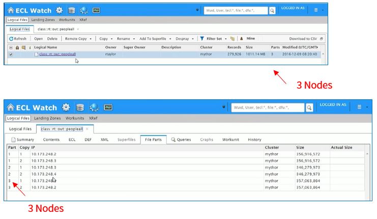
The file “~class::rt::out::peopleall” will be used in all examples. 

In ECL Watch, we see that the data is distributed over 3 nodes.

Example 1:

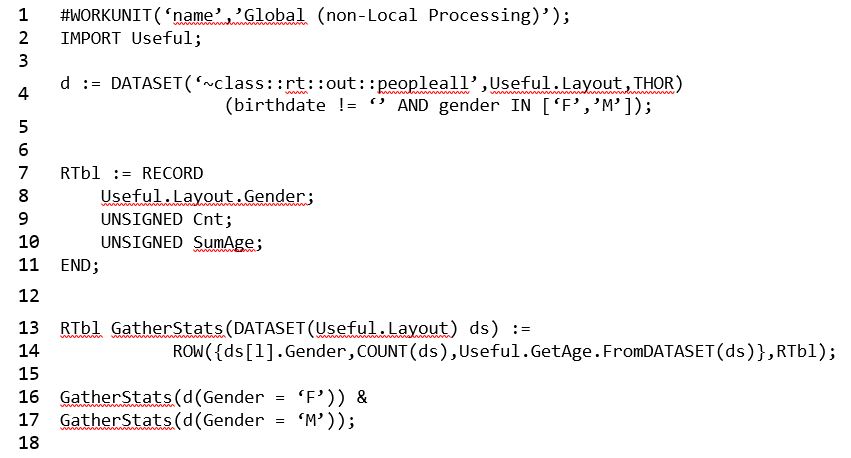
In Example 1:

• DISTRIBUTE has not been applied to this workunit. The DISTRIBUTE function is used to distribute data evenly across all nodes in a cluster.
• On line 4, the dataset is defined using birthdate and gender.
• On line 14, a row is generated that is filtered by gender, counts the number of males and females, and sums their ages.
• Lines 16 and 17 pass two datasets filtered for female and male respectively, and generate a dataset from those two rows using the ampersand (&).
• Using GLOBAL processing, a results table is generated that shows count by gender, and a sum of the ages.

Results (Example 1):

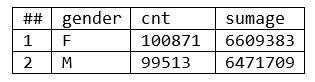
***In this instance, the dataset is small, so there is no “cluster skew.”  For a larger dataset, “cluster skew” could be a problem.

Example 2 – Using the TABLE Function with LOCAL Results

In this example, the same calculations as those in the previous example are executed using the TABLE function and a LOCAL qualifier.

Example 2:

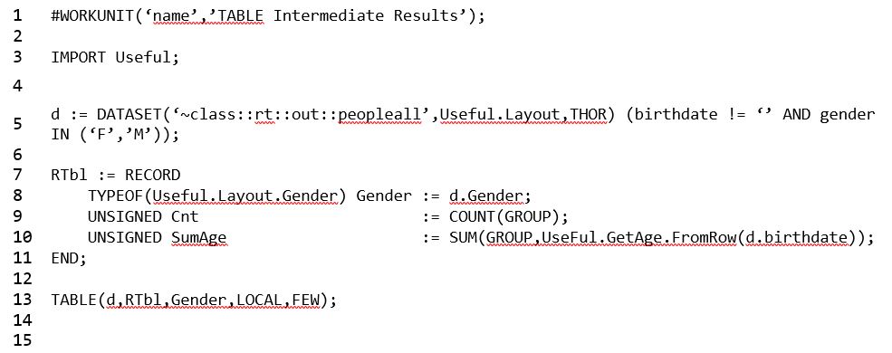
• On line 13, the LOCAL qualifier is applied to the TABLE command, so the TABLE command will execute independently on each node.

Results (Example 2)

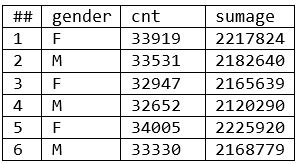
• The results table shows count by gender (cnt), and a sum of the ages (sumage).
• There are six results (two results per node), with data grouped by node and gender.
• The inputs and outputs are the same as the prior example (example 1), but this summary includes intermediate results. There is one more phase to complete; the results must be amalgamated into a final result. (If you add up the counts and sumages by gender, you will get the same results as example 1).

Example 3 – Using the TABLE and ROLLUP Functions with GLOBAL Results

Example 3 is similar to example 2, with a couple of additional steps: the addition of ROLLUP and GROUP functions.

Example 3:

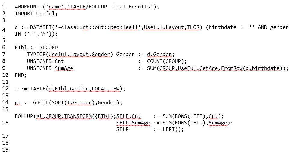
• On line 12, a LOCAL qualifier is applied to the TABLE function.
• On line 14, the dataset is grouped by gender.
• On line 15, the ROLLUP function is applied, which provides final results instead of intermediate results. 

Results (Example 3)

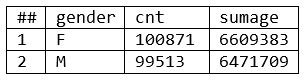
• The results here are the same as the results for example 1, but the compiler runs in a fraction of the time, and avoids “cluster skew.”

So far, we have summarized the dataset using the TABLE and ROLLUP functions. Next we will gather and summarize data using the AGGREGATE function. 

The syntax for the AGGREGATE function is the following:

AGGREGATE (recordset, resultrec, maintransform [, mergetransform (RIGHT1, RIGHT2)] [, groupingfields]

There are two types of TRANSFORM functions listed within the syntax of the AGGREGATE function: maintransform and mergetransform. The maintrasform calls for each matching pair of records in a recordset, and the mergetransform calls to merge the result records of the maintransform. Before diving deeper into the AGGREGATE function, let’s discuss the requirements for the TRANFORMs.

AGGREGATE TRANSFORM Function Requirements

The maintransform must take at least two parameters: a LEFT record of the same format as the input recordset and a RIGHT record of the same format as the resultrec. The format of the resulting record set must be the resultrec. LEFT refers to the next input record and RIGHT the result of the previous transform.

The mergetransform must take at least two parameters: RIGHT1 and RIGHT2 records of the same format as the resultrec. The format of the resulting record set must be the resultrec. RIGHT1 refers to the result of the maintransform on one node and RIGHT2 the result of the maintransform on another.

The mergetransform is generated for expressions of the form: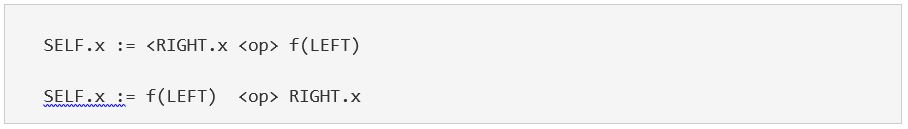

where the <op> is: MAX, MIN, SUM, +, &, |, ^, *

Now that we’ve looked at the requirements for AGGREGATE TRANSFORMs, let’s examine how AGGREGATE is applied.

Example 4 – AGGREGATE with Local Results

In example 3, two built in functions (TABLE and ROLLUP), along with the GROUP function are used together to gather and summarize the data. Example 4 demonstrates that AGGREGATE is a “one stop shop” for data gathering and summarization. 

Example 4: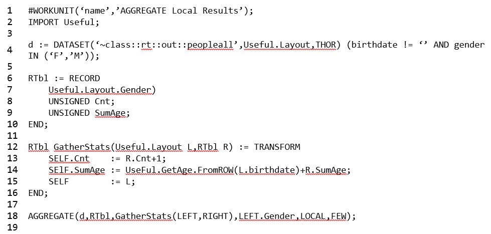

• Note that it is not necessary to DISTRIBUTE data before using AGGREGATE. Refer to the blog ECL Tip – DISTRIBUTE for a detailed explanation of DISTRIBUTE.
• On line 18, LOCAL used with AGGREGATE operates like the TABLE function. In this instance, it tells the compiler not to complete the final phase (summarizing results).

Results (Example 4):

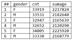
• The results are identical to those in example 2, where the TABLE function with a LOCAL qualifier was used. The main difference between the AGGREGATE and TABLE functions is that TRANSFORM is used with the AGGREGATE function, and a RECORD layout is used with the TABLE function.

Example 5 – AGGREGATE with GLOBAL Results

In this example the LOCAL command is removed from the AGGREGATE function (line 18), so the results are GLOBAL.

Example 5:

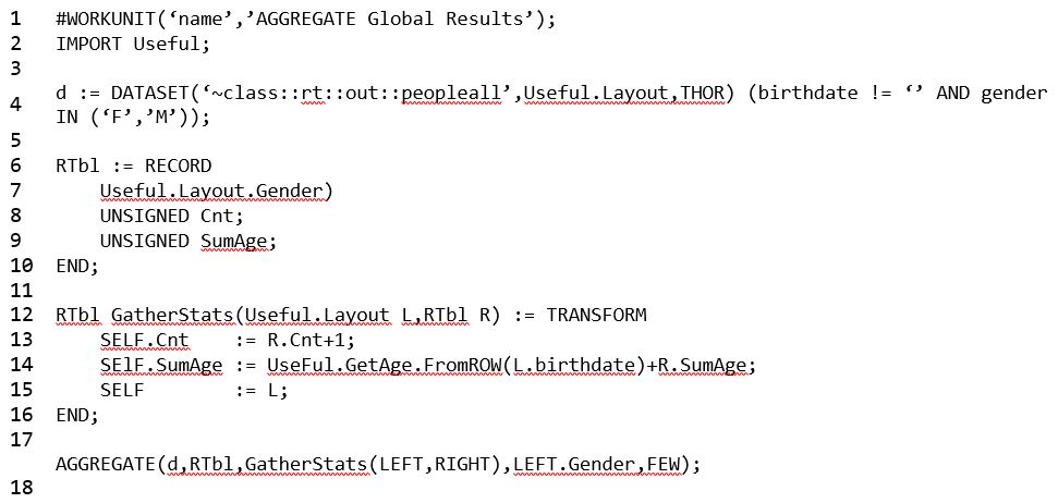
• The compiler deduced the second phase (merge operation) from the format of the maintransform (line 12), so there is no need to specify a second TRANSFORM. A second TRANFORM can be specified, but is not necessary.
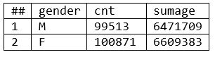
• The results below are identical to the results for the globally-run workunits in prior examples.

Results (Example 5):

 

 

Example 6 – AGGREGATE Demo with 2nd Transform

This example demonstrates what happens when a second TRANSFORM is added, and the results are fed LEFT side of future iterations.

Example 6:

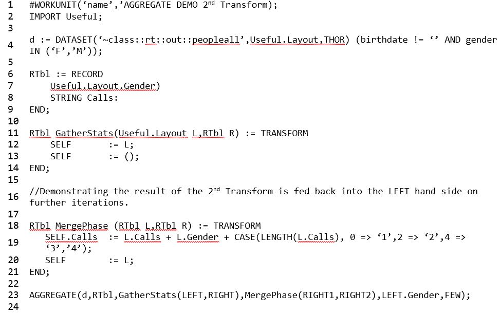
• On line 4, for this dataset, the male gender is represented by ‘M’ and the female gender is represented by ‘F.’
• On line 19, the MergePhase TRANSFORM represents the results of each iteration in “lengths,” with the first length = 0, the second length = 2, and so on.  Each iteration for this string is accumulated.
• On line 19, the string calls the first TRANSFORM (line 11). The length of the call for the first iteration is 1 (0 => ‘1’), and the length of the call for the 2nd iteration is 2 (2 => ‘2’).
• On line 19, the mergetransform takes the left hand side (L.Calls) of the first TRANSFORM (line 11) and passes the result recordset from the iteration.

Results (Example 6):

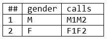
• These results show that in “MergePhase(RIGHT1,RIGHT2),” RIGHT1 holds the intermediate results. So M1 and F1 represent intermediate results, and M2 and F2 represent final results.

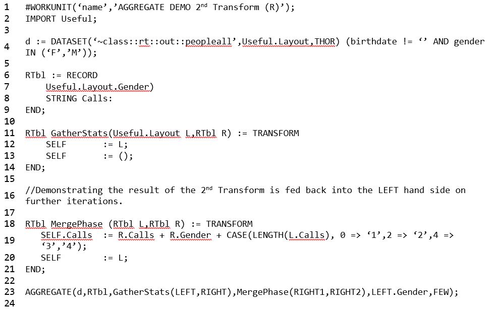
Example 7 – AGGREGATE Demo with 2nd Transform (R)

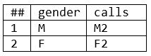
If we duplicate example 6 using the right side (reference line 19), information from each iteration is not accumulated, which generates a table with final results.

Results (Example 7):

Summary

In this blog, we gave of examples of ways to gather and summarize data. We gave an example of “what not to do,” along with examples of how the TABLE and ROLLUP functions are used. We also discussed the ECL AGGREGATE function and provided examples of how the function is applied.

For access to Allan Wrobel’s Tech Talk video, please use the following link: Tech Talk 23 – Leveraging the Power of HPCC Systems – Use AGGREGATE

About Allan Wrobel

Allan has worked in the IT industry since 1976 (and still has some old punch cards to prove it). Really too many avenues and technologies to enumerate here, but has tended to gravitate to the construction and analysis of databases.

He now has a rather jaundiced view of the ‘latest thing’, given we were most probably working on much the same in 1982. Allan’s world view and HPCC seems to coincide quite nicely, to an extent that he’s become a quite a prophet (one of the minor ones)  for HPCC and ECL and has a growing YouTube playlist available to all without the annoying 6 second ads.

Acknowledgements

A special thank you goes to Allan Wrobel for his informative presentation on the ECL AGGREGATE Function.