Reproducing Kernel Hilbert Space (RKHS) — A primer for non-mathematicians
Reproducing Kernel Hilbert Spaces (RKHS)
While working on the Causality 2021 project (see details here), we found that the most powerful and performant algorithms for statistical methods tend to be based around RKHSs. So we set out to understand what they are and how to apply them, which led us into a deep pool of mathematics that was a long way above our heads. Nonetheless, we had to get to the other side, so we dog-paddled our way across with the help of many difficult papers that gradually let us understand each of the concepts prerequisite to RKHS.
It turns out that RKHS are a very useful tool to have available, with many really nice characteristics for many types of algorithm. In the learning process, I’ve been able to understand most of the math behind it, and will attempt to distill it into terms more accessible to engineers, and hopefully save others the painful journey.
Note that my description will, necessarily, lack full mathematical rigor, and may lead to some statements that are not quite technically correct. But that’s the price of easy understanding. Once the basics are understood, the follow-on details become much easier to absorb.
What are they good for?
Let’s start with: what are they good for? If it hadn’t been for the successful algorithms built using RKHS, I would never have gleaned their usefulness from reading the descriptions, and would not have never taken the time and effort to learn them.
RKHS have a broad set of applications in the analysis of data. They are commonly used in Machine Learning algorithms, where they are known as “kernel methods”. In that context, they translate data into a higher (often infinite) dimensional space, where it is far easier to separate data points than in their native space. But there are many other types of application:
Statistical Methods — RKHS are used to perform approximations of difficult statistical calculations such as Independence, Conditional Independence, and Conditional Probability. These are the applications that drew me to learn about them. The RKHS algorithms were always the most accurate, and had much better scaling properties with increasing data size and problem dimensionality. In fact, some RKHS algorithms allow linear scaling with data size, while traditional approaches scale quadratically or cubically[4].
Other Applications:
- Signal Detection — RKHS are agile at separating signal from noise in communication settings.
- Function Emulation — RKHS can perform the hat trick of converting a discrete set of measurements into a continuous function. This can be used, for example, to determine a Probability Density Function or a Cumulative Density Function associated with any sized data set.
- Future Applications — RKHS are very flexible, and many other applications will surely be discovered.
What is an RKHS?
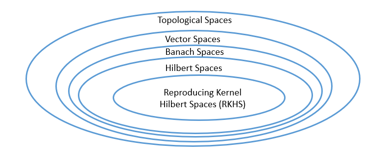
Mathematically, RKHSs are a specific type of topological space with some very handy and surprising characteristics. It is almost impossible to imagine the shape of most RKHS spaces. They are typically very non-linear, and high to infinite dimensional. But here are some of the practical implications.
- It is a space of functions.
- Each point in space is a particular function.
- Function spaces tend to be infinite dimensional, so not only are there an infinite set of functions there, but the vector that identifies a given function can be of arbitrary (theoretically even infinite) length.
- Your sample data is typically used as the index into the function space. Index entries are real-valued.
- The functions are organized locally such that if the indices are similar, the resulting functions will be similar.
- The functions are smooth and continuous. Each function takes a single real-valued parameter, and returns a single real value.
- Linear functions in RKHS provide useful non-linear results. This is the unique characteristic of RKHS that makes it so useful.
- RKHSs are identified by a unique “kernel function”. Each kernel induces exactly one RKHS, and each RKHS has a unique kernel function.
One common use of RKHS is to find a function that describes a given variable. The data (samples of that variable) is given as the index into the function, and the function returned will estimate the probability density of the data’s generating function. It is guaranteed to converge to the exact function that generated the data as the number of data points approaches infinity (with a few caveats*). Better than that, it will approach the correct distribution with every additional data point. Better still, every prediction that that function returns will be close to the actual value.
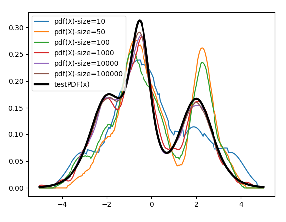
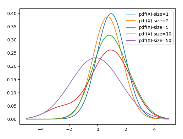
The plot below shows a variable that is a random mixture (mixture model) of three different Logistic Distributions. Samples of various sizes are given to the RKHS. Note that even with small amounts of data — see blue line with only 10 data points — the RKHS produces a decent facsimile of the distribution, and that the approximation gets ever closer as the amount of data increases.
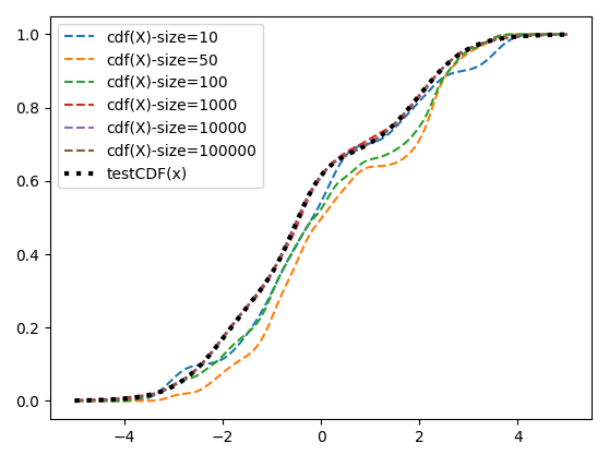
By changing the kernel function, we can create the same graph for the Cumulative Density function of the same distribution.
In fact, the function returned from the RKHS can be almost any function of the mechanism that generated the data. The meaning of the result is controlled by the kernel.
If the above wasn’t good enough, there are many techniques that allow acceleration of RKHSs, via approximation. Fast approximations can be made that will always be in the direction of the desired function, and with very little error.
The kernel of the RKHS determines what types of function are available in the space, as well as the meaning of the function’s result. Different kernels produce different types of functions, but some kernels are universal, meaning that they can emulate any continuous function to within isometric isomorphism, which is a fancy way of saying “exactly the same on the outside, though it may be different inside”.
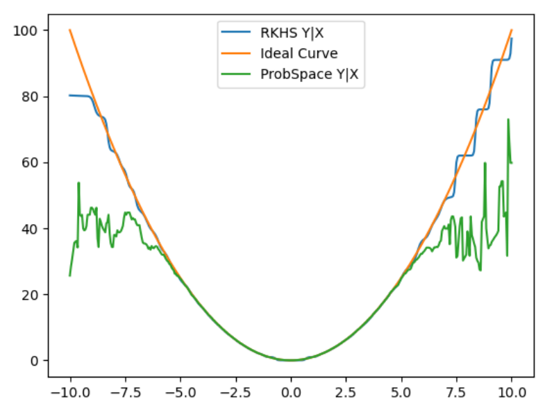
If we think about the key problem of Conditional Probability, it is that in order to condition on multiple variables and get an exact answer, we need exponentially more data with the size of the conditioning set. In any real-world scenario, we will quickly run out of data when we need to condition on many variables. RKHS solves this problem by returning a continuous function that represents the distribution, meaning that we effectively have an infinite number of data points to work with.
The plot below compares a computation of conditional probability based on traditional methods vs RKHS. Even with only a single conditioning variable, we have very little data out on the tails of the distribution, and the computations quickly break down. The RKHS version is able to closely follow the ideal results, way out into the distributions’ tails.
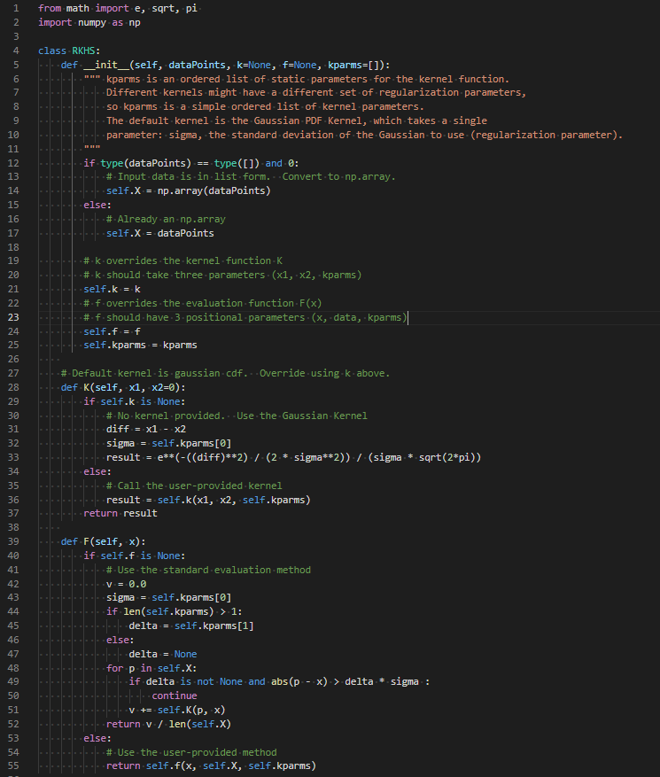
Now I’ll share a secret about RKHS that you will seldom see exposed in any papers or articles. Implementing RKHS is embarrassingly easy. It may take hundreds of pages of math to describe RKHS, but only a few lines of code to make it work. The code sample at the bottom implements a flexible, optimized RKHS in under 30 lines of Python code. A hard coded RKHS could probably be done in 10 lines. It bothers me that it took several weeks of intense study to understand an algorithm that took me an hour to implement. That’s what motivated me to write this article.
* The major caveat is that the function has to exist within that particular Hilbert Space. Not every possible function necessarily exists in a given Hilbert Space. For example, my sawtooth kernel space may not contain (even in infinite dimension) the exact function for a Logistic distribution. But that doesn’t stop it from being used to emulate one. Certain kernels, such as the Gaussian Kernel are proven to be “universal”, or “infinitely smooth”, meaning that the Hilbert Space the kernel induces contains all continuous functions.
How does it actually work?
As you read the articles on RKHS, it seems like a sort of black magic. How can it all possibly work? Well, as the trivial code might indicate, the mechanism is also very simple.
I discussed the kernel above, but not any function can be a kernel. The kernel requires some basic characteristics in order to be valid. It is a function that takes one or two values, and serves two distinct purposes: When presented two arguments, it returns a distance in Hilbert Space between the two arguments, and when presented a single argument, it translates that argument into the Hilbert Space.
The requirements for a kernel function are:
- Symmetry — K(A,B) = K(B,A)
- Positive Semi-Definiteness — This just means that it always produces a positive (i.e. > 0) result, except in the case where the inputs are zero.
- Square Integrability — A fancy way of saying that the function is well-behaved. It doesn’t have discontinuities, and doesn’t veer off into infinity.
- It is computed by taking an inner product of its parameter with the data provided to the RKHS.
The only other structure within an RKHS is the evaluation function F(x), which is the function produced given the data. This is, in many cases, just: sum(K(xi, Data[i])) for all i in range(n)) / n, where n is the number of data points in your sample. This is also known as the RKHS mean.
Let’s look at Figure 2, which is a very simple application of RKHS. My kernel is:
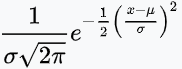
which, if it looks familiar, is the Probability Density Function (PDF) of a normal distribution. This is known as a Gaussian Kernel, and has been shown to be “universal”, meaning it can emulate any curve. It is particularly good for statistical functions since all distributions when added together approach a Gaussian (normal) distribution.
Let’s look at a very simple test, that calculates the PDF of a single Logistic Distribution with mean = 0 and scale = 1. If we give this RKHS a single sample data point, it will produce a Normal curve with mean at that point. In this case, our first sample (rounded) was .96, so it approximated our Logistic(0,1) with a Normal(.96, sigma), where sigma is a regularization parameter set to 1 in this example.
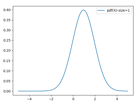
While this is not a very good approximation, it’s not too bad for exactly one example.
Now as we add a second point, in this case, .47, it creates a second Normal curve, this time with a mean of .47. It averages the two together, which forms a new approximation (orange line). This approximation is getting closer to the actual mean of zero.
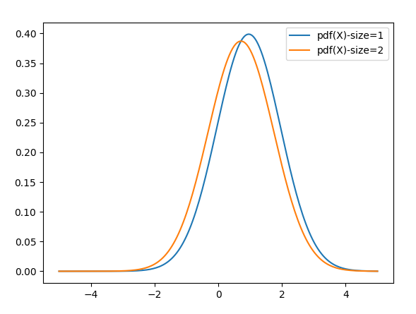
As I add more data points, the same process occurs. Each new Normal curve is averaged with the others producing the function that is just an average of Normal curves. As more and more points are added, this average will approach the generating function surely. An average of enough Normal curves can identically produce any other curve of any complexity as the number of data points approaches infinity. Note below that the purple curve (with 50 points) has already come close to the correct mean of zero. Although the difference is not detectable by eye, the resulting form is no longer Normal, but is approaching the shape of a Logistic Distribution.
Lest you think that there is some magic hidden in the Normal (Gaussian) Distribution, look what happens when I change kernels, and simply put a triangle where each Gaussian was previously placed, using this “sawtooth” kernel function.
K(x1, x2=0) = max(0, (1 – (abs(x1 – x2) * P))) * P
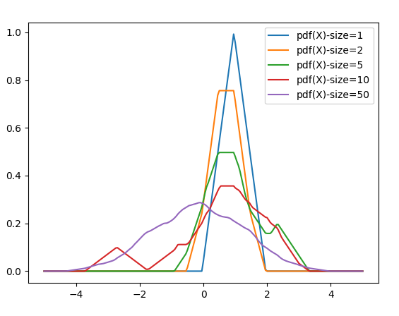
Notice that with one data point, an Isosceles triangle was placed with its point at that position. By the time we had 50 data points, it had come close to the zero mean, and started to approach the shape of a Logistic Distribution.
So does it matter what kernel we choose? It does indeed. While almost any valid kernel (a square, a truncated triangle, etc.) will approach the correct result, they don’t all approach as smoothly or as quickly. It might take my sawtooth kernel 500 points before it starts to really resemble a Logistic Distribution, while the Gaussian gets there in 50. So choice of kernel does matter, but there’s no magic in any kernel. While it is easy to create a kernel, it is notably difficult to find an “excellent” kernel for a given application. There are many “excellent” kernels that have been found for various tasks, such as the Gaussian or Radial Basis Function (RBF) kernel, the Fourier Kernel, and others. Kernels have been developed for specialized tasks such as analyzing graph relationships, or images. But for basic numbers, and especially statistics, the Gaussian is hard to beat.
Linearity of Operations
My final topic in this primer is a very important feature of RKHS, and that is linearity of operations. The RKHS behaves in many ways like normal Euclidean space. This means that if we apply linear methods in RKHS, they change their meaning in a very important way. A linear regression in RKHS is equivalent to a non-linear regression in a complex infinite dimensional space. So points that can’t be separated by a line (or hyperplane) in their native space can be easily separated by a linear regression in RKSH. Similarly, if we compute function of variables in Euclidean space, such as Correlation(A,B), it tells us if the variables are linearly related. A Correlation of 0 indicates that the variables are linearly independent. If I do the same calculation in RKHS, it tells me if the variables are Independent (i.e. non-linearly uncorrelated). The same is true with nearly any linear operation — in RKHS it becomes a non-linear operation. This is exemplified by the use of “kernel methods” in machine learning, though there are many other similar uses.
Conclusion
RKHS is an important technology. It is notoriously difficult to learn, but embarrassingly easy to use. Although the math has been available for nearly 120 years, its use has been limited due to its abstractness. I hope I managed to explain RKHS in a less technical way without the difficult mathematical notation, theorems, and proofs. My goal was to make RKHS more accessible and less daunting, and encourage you to try it for your own algorithms. I hope I’ve succeeded to some degree. Let me know if you find new, innovative ways to apply RKHS. If you are intrigued by RKHS and you’d like to understand the math behind it, [1] below provides a thorough “Primer” on the subject. Be forewarned that it is 80 pages of difficult reading, but it covers all relevant aspects, and several applications. In any event, it will surely cure insomnia. It worked for me!
References
[1] Manton, Jonathan H; Amblard, Pierre-Olivier (2015) “A Primer on Reproducing Kernel Hilbert Spaces”, Foundations and Trends in Signal Processing. URL: https://arxiv.org/pdf/1408.0952.pdf
[2] Sriperumbudur, Bharath K.; Gretton, Arthur; Fukumizu, Kenji; Lanckriet, Gert; Scholkopf, Bernhard (2008) “Injective Hilbert Space Embeddings of Probability Measures”, Conference on Learning Theory, URL: http://www.learningtheory.org/colt2008/papers/103-Sriperumbudur.pdf.
[3] Smola, Alex; Gretton, Arthur; Song, Le; Scholkopf, Bernhard (2007) “A Hilbert Space Embedding for Distributions”, URL: http://www.gatsby.ucl.ac.uk/~gretton/papers/SmoGreSonSch07.pdf.
[4] Rahimi, Ali; Recht Ben (2007) “Random Features for Large-Scale Kernel Machines”, NIPS’07: Proceedings of the 20th International Conference on Neural Information Processing Systems, December 2007 Pages 1177–1184.
Appendix A — Python Code
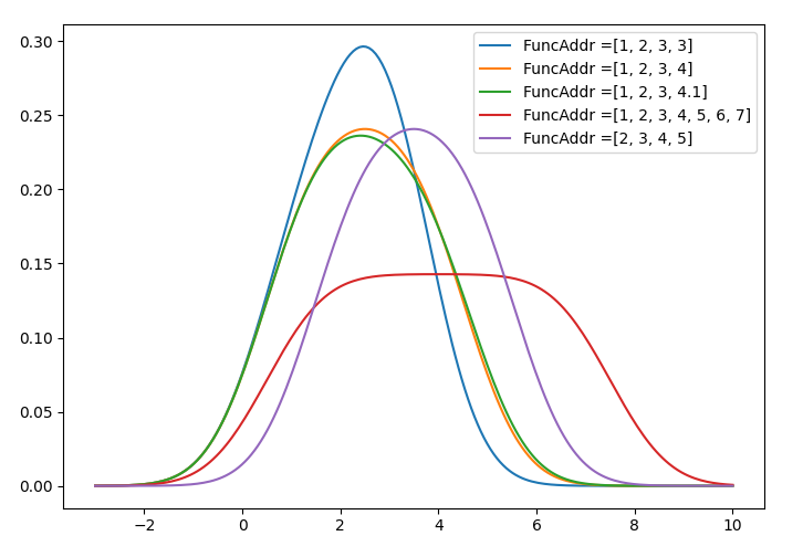
Earlier in the article I talked about indexing into the infinite set of functions in the RKHS. In practice, your data is the index into your function space. But just to illustrate notions of function locality, and to provide a simple example, we will look at functions with various indexes that are close or far from each other.
Here is the output:
The code below can be found in the working repository here.
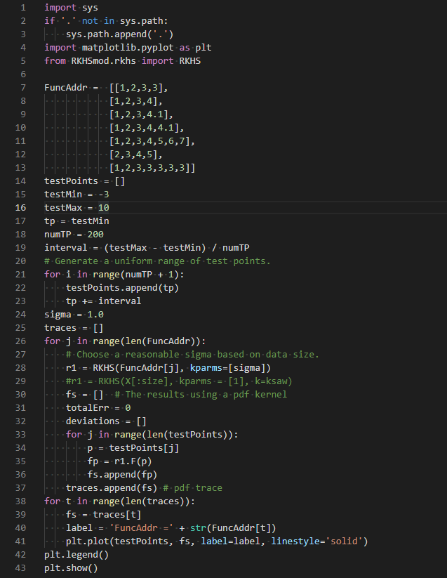
The following test code generated the graph above:
RKHSmod/rkhsTest3.py
Here is the code for the generalized RKHS:
RKHSmod/rkhs.py