Soccer Analytics: Leveraging Raw GPS Data for Optimizing Player Performance
Introduction
In today’s world, Data Analytics is an important part of sports. Sports organizations on every level use data analytics to predict and improve player performance, a team’s quality of play, prevent injury, increase revenue, and more. Christopher Connelly, a Sport Scientist at North Carolina State University (NCSU), spoke at Community Day 2019 and HPCC Systems Tech Talk 29 about the university’s Athlete 360 program.
For the Athlete 360 program, Python, SQL, and HPCC Systems are used to build programs and a database that support an athlete data monitoring platform for the Strength and Conditioning department. GPS data is collected with the help of the NCSU men’s and women’s soccer teams, which is then processed and analyzed using HPCC Systems.
In this blog we discuss the details of the Athlete 360 program, including data sources, methodology, and data analysis. Examples of the data analysis include, typical movement patterns for certain drills or differences between positions, distances for typical efforts at different speeds and distance recorded in GPS data for a specific effort against a known distance.
Let’s begin by discussing data sources and the Athlete Management System.
Sources of Data
Sources of data for the Athlete 360 project include:
- Spreadsheets –The spreadsheets provide information on what a player is doing on field with the team, what they are doing in the gym, how they’re playing in their games, results of those games.
- Exercise Equipment
- Workouts
- Competitions
- Personal Fitness Devices
Athlete Management System
The goal of the Athlete Management System is to:
- Collect data in one place
- Analyze data
- Predict outcomes
In the Athletic Management System data sources are brought together into one place to get a big picture of what is happening, data is analyzed to determine how everything is interconnected, and analytics are used to predict player performance in various scenarios. This helps coaches and trainers optimize training programs and game plans for the athletes.
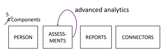
The five components of the Athletic Management System are shown in the graphic below. This system consists of the athlete, assessments that are used to collect data, reports that go back to the coaches, connectors that connect all of the data sources together for analysis, and advanced analytics to find trends over time, or any type of relationship between variables that give insight into player performance.
The Data
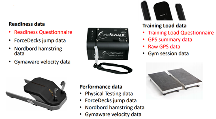
The data for the Athlete 360 program is divided into three types:
Readiness Data – Readiness data is provided several times a week, and compares athlete performance against his/her normal baseline.
- Readiness Questionnaire – Provides a subjective rating based on how athletes feel on a particular day, and how they are responding to training.
- ForceDecks Jump Data – ForceDecks are force plates that allow testing, analysis and interpretation of athlete data.
- NordBoard Hamstring Data – NordBoard is a system that measures hamstring strength and imbalance
- Gymaware Velocity Data – Gymaware is a small, portable, and accurate linear encoder that attaches to free weights bars and weight stack machines for measuring Power output
Training Load Data – Allows the athlete to see and track the amount of strain placed on the body as a result of recorded activities over time.
- Training Load Questionnaire – Questionnaire completed after every gym training or practice session. Asks what the athlete experienced during that session, and how they rate their effort and their exertion.
- GPS Summary Data
- Raw GPS Data
- Gym Session Data
Performance Data – Compares practice and training load data to physical testing and measures that assess on-field performance capabilities.
- Physical Testing Data
- ForceDecks Jump Data
- NordBoard Hamstring Data
- Gymaware Velocity Data
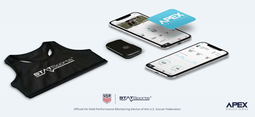
STATSports Apex
The STATSports Apex system is used to gather GPS data during practice sessions out on the field. This systems tracks key metrics, such as maximum speed, total distance, and high speed running. The package includes a GPS Performance Pod, Apex vest, and Apex Athlete series app.
The image below shows a beacon (Apex) used to track data in real time during practice sessions. The iPad software tracks key metrics during practice sessions.
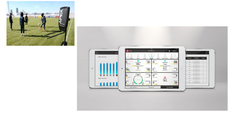
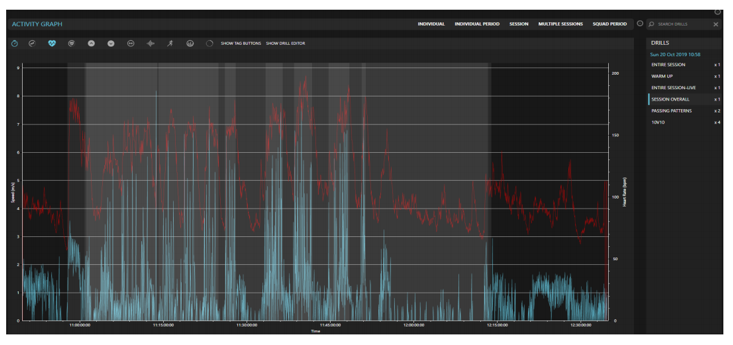
STATSports Dashboard
The STATSports Dashboard displays a view of the data from the GPS. This view enables the user to organize practice session data.
System Setup
Below are the steps used to gather, process, and analyze data for the Athlete 360 program:
1) Pull data from various sources to local storage.
2) Upload data to the landing zone through ECL watch, using HPCC Systems.
3) Spray data onto the cluster.
4) Run ECL program to clean and process data based on set layouts.
5) Run ECL programs to manipulate data for necessary variables.
6) Despray data from cluster to landing zone.
7) Upload data to tables created in ClickHouse.
– ClickHouse is an open-source column-oriented database management system that allows the generation of analytical data reports in real-time, using SQL.
8) Perform queries on ClickHouse tables in Redash to display the most recent data in pre-made dashboards.
– Redash is an open-source SaaS application used to query data sources, visualize the results, create visual dashboards, and share
Data Flow
The diagram below was created in Tombolo, and shows the flow of data for the Athlete 360 project. This diagram gives a view of the GPS data received for two soccer teams, and how it is organized to give an overall view of everything that will affect the athletes. The highlighted portion is the data that will be used in subsequent examples.
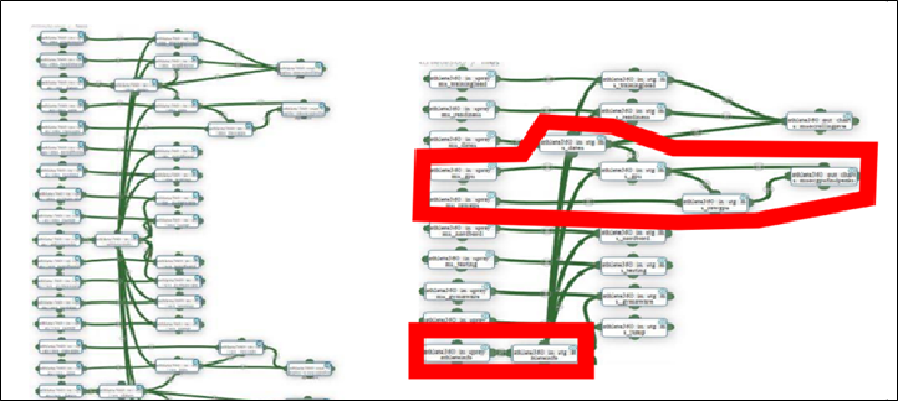
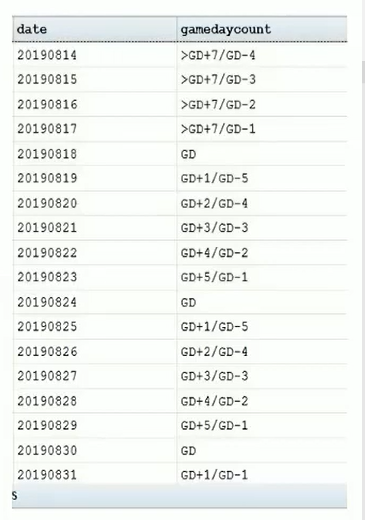
The GPS data is paired with a data file that gives all possible dates for given time periods, and allows the user to categorize and compare the type of day (practice session, drill, strength training, game, etc.). The bottom area highlighted in red is the athlete info file. This file tells us the team each athlete is a part of, the positions these athletes play, the year they graduate, and any unique identifiers for the athletes.
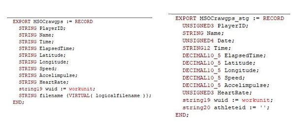
Example of data processing/manipulation
This is a view of how the data is organized when it is uploaded to HPCC. These are the data fields with field names, and the appropriate data types. As data is processed, the athlete ID is used to identify each athlete and connect to various data sources.
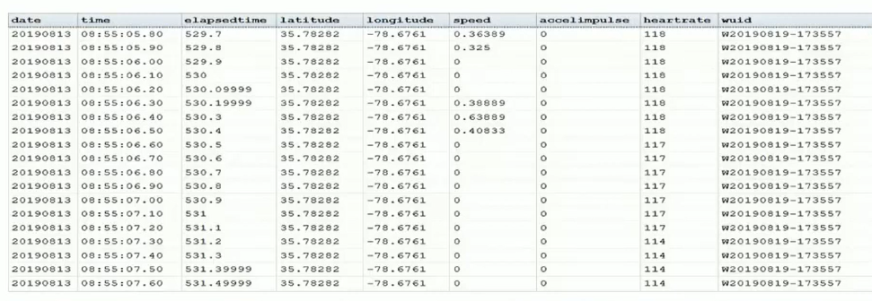
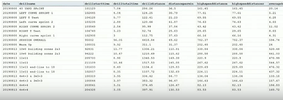
Aggregated Data from GPS Data
These tables show aggregated data from the GPS software that list the names of all practice drills, start times, and durations of the drills. The top table is the raw GPS data, and the table underneath is a summary of the GPS data. It is also possible to display player position and type of day. Layering all this information together on to the raw data gives the context needed to determine the best data analysis methodology.
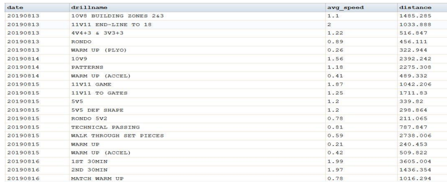
Example: Average Distance
This is an example of how information is extracted from raw GPS data. In this portion of code, the aim is to get an average distance for a specific drill period on a specific day. The bottom table shows data for an athlete over several days. Various drills are shown with dates, average speeds, and distances.
The information extracted includes a breakdown of each part of a practice where the most distance is covered, and where the highest average speeds are achieved. This gives an idea of the most intense part of practice, and the part of practice with the heaviest workload. These results are then compared to other days that have similar drills, to get an idea of the workload for specific drills.
DATA_DISTANCE := SORT(
TABLE(completegpsdata,
(name, date, drillname,
decimal5_2 avg_speed := AVE(group, speed);
decimal8_3 distance := AVE(group, speed) * (MAX(group, elapsedtime) – MIN(Group,elapsedtime));
},
name, date, drillname,
MERGE
), name, date, drillname
);
Example: Average Heart Rates
In this example, the goal is to determine average heart rates for 1 minute, 3 minute, and five minute time periods, based on the number of rows of data. For the one minute interval, at ten data points per second, the result is 600 rows of data. The 3 minute time period gives 1800 rows of data, and the 5 minute time period results in 3000 rows of data.
The results enable the user to determine which time period for a specific drill has the highest average heart rate. The 1 minute intervals normally have short bursts of activity, so the average heart rates are lower. The five-minute time periods have more sustained effort, so the average heart rates are higher. In this instance, there will be higher heart rates for a longer period of time. If they do not sustain those efforts there will be more spikes in the heart rate data. Those shorter drills that show high heart rates are not expected to last for as big of a window of time, but it gives the user an idea of the intensity of the drills.
lay1 iterateme(lay1 L, lay1 R, integer cntr) := transform
SELF.cnt := IF(cntr = 1 or L.name <> R.name or L.date <> R.date, 1, L.cnt + 1),
self.speedsumval := IF(SELF.cnt = 1, r.speed, L.speedsumval + R.speed);
self.hrsumval := IF(SELF.cnt = 1, r.heartrate, L.hrsumval + r.heartrate);
self := R;// IF(SELF.cnt = 1, R, L);
end;
rawDSsums := Iterate(rawDs3, iterateme(LEFT, RIGHT, COUNTER));
//add fields that will be used to create the 1 min periods
rawDSsums_limit1 := JOIN(
rawDSsums,
rawDSsums,
left.name = right.name, and left.date = right.date and left.cnt-600 = right.cnt,
transform(
(recordof(left), decimal10_5 sumspeedlimit1, integer sumhrlimit1},
SELF.sumspeedlimit1 := IF(right.name = ‘’, LEFT.speedsumval, LEFT.speedsumval – right.speedsumval);
SELF.sumhrlimit1 := IF(right.name = ‘’, LEFT.hrsumval, LEFT.hrsumval – right.hrsumval);
SELF := LEFT
),
LEFT OUTER,
LOOKUP
//add fields that will be used to create the averages
rawDSaves := Project(rawDSsums_limit5,
transform(
{RECORDOF(LEFT), decimal10_5 speedave1, decimal10_5 speedave3, decimal10_5 speedave5,
decimal10_5 hrave1, decimal10_5 hrave3, decimal10_5 hrave5},
self.speedave1 := left.sumspeedlimit1/600;
self.hrave1 := left.sumhrlimit1/600;
self.speedave3 := left.sumspeedlimit1/1800;
self.hrave3 := left.sumhrlimit1/1800;
self.speedave5 := left.sumspeedlimit1/3000;
self.hrave5 := left.sumhrlimit1/3000;
SElF := LEFT;
));
Example: Game Buckets
In this example, a game is broken up into 15 minute segments, denoted by bucket numbers (“bucketnum”). There are 3 buckets per half in a game, but occasionally there will be a fourth bucket to account for “spill over” time. In soccer, extra time is allotted for stoppages and other things that prolong the game.
The coaches are able to evaluate various details of the game using this data – observing how the athletes progress during the game, looking for trends between games, determining how well strategies work, and comparing with other games.
lay1 iterateme(lay1 L, lay1 R, integer cntr) := transform
self.drillstarttime_new :=
IF(cntr = 1 or L.name <> R.name or L.date <> R.date or L.drillname <> R.drillname,
r.drillstarttime,
L.drillstarttime_new);
Self := R;// IF(SELF.cnt = 1, R, L);
End;
rawDSsums := Iterate(newdata, iterateme(LEFT, RIGHT, COUNTER));
finalResult := PROJECT( rawDSsums,
transform(recordof(left),
self.bucketnum := Athlete360.util.get_gametimebuckets(left.drillstarttime_new,Std.date.
FromStringToTime(left.time(1..5),’%M:%M:%S’));
SELF := LEFT
)
);
DATA_DISTANCE := SORT(
TABLE(finalResult,
(name, date, Position, drillname, bucketnum,
decimal5_2 avg_speed := AVE(group, speed);
decimal5_3 distance := AVE(group, speed) = (MAX(group, elapsedtime) – MIN(Group, elapsedtime));
decimal5_3 time_diff := ((MAX(group, elapsedtime) – MIN(Group, elapsedtime))/60);
),
name, date, Position, drillname, bucketnum,
MERGE
), name, date, Position, drillname, bucketnum
);
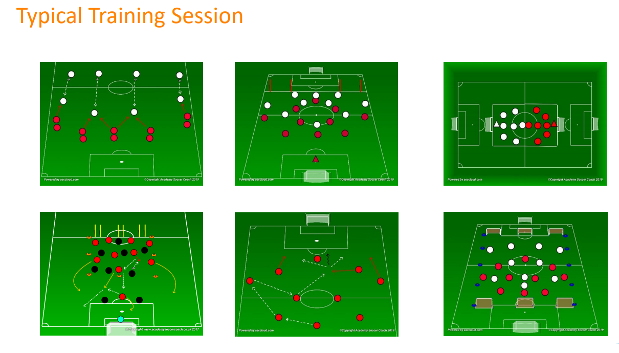
Example: Data Analytics for Practice Sessions
There are many different types of drills in a typical practice session. Data for these practice sessions can be overwhelming and confusing. Data analytics and reporting allow the user to break down those practice sessions and help make sense of the data, reporting it back to coaches in a way that will help them understand it better. This allows the coaches to prove or disprove that the intent of the training session was met, making adjustments where necessary.
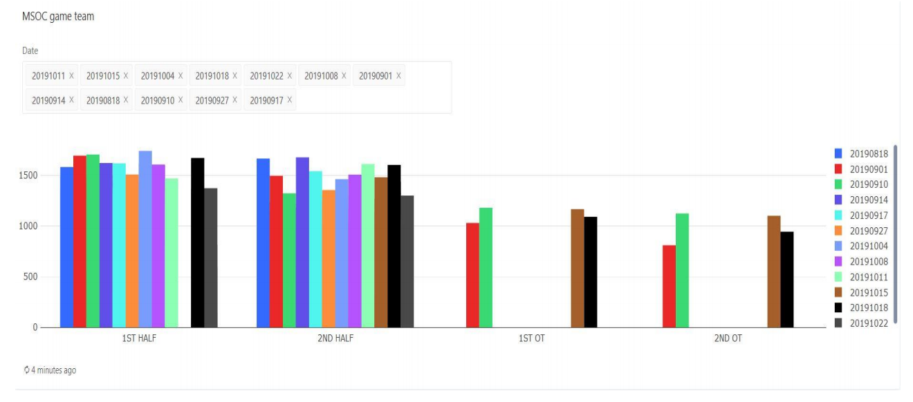
Example: Game Breakdown with Distance Covered for Each Player
This graph gives a breakdown of every game played this year, with distance covered during each section of that game. This enables the coaches to determine player performance from game to game. The coaches are able to see player progression throughout the season.
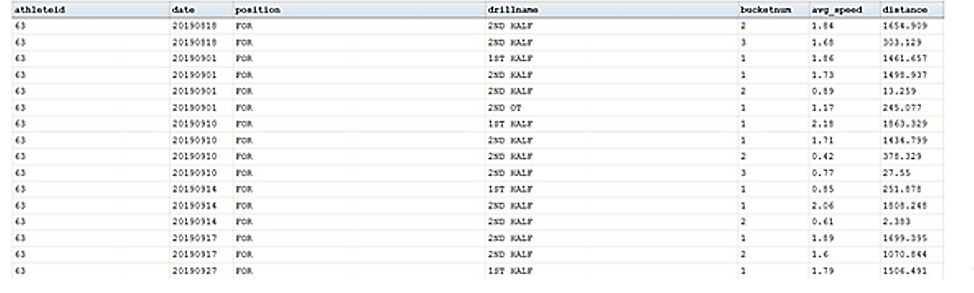
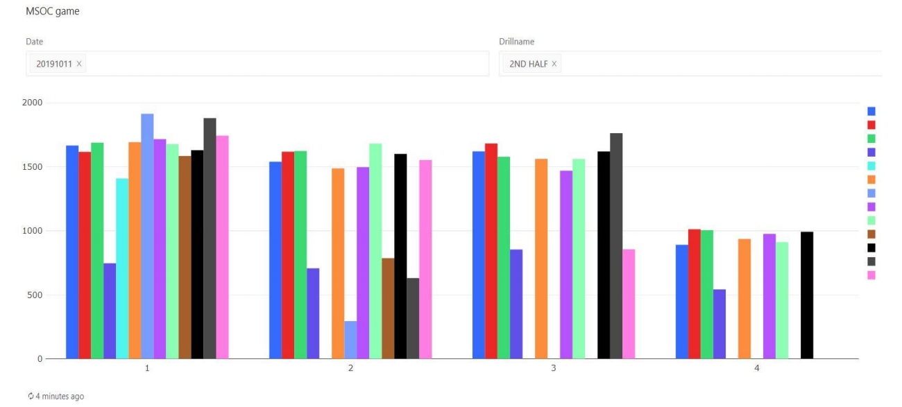
Example: Game Data by Position and Player
This graph shows the second half of a game, broken down by buckets (15 minute segments) and player discipline. It also includes “spillover time” and distances covered. This view allows for comparisons between different players at a specific position, during a specific period of time. It also allows for comparisons between different positions.
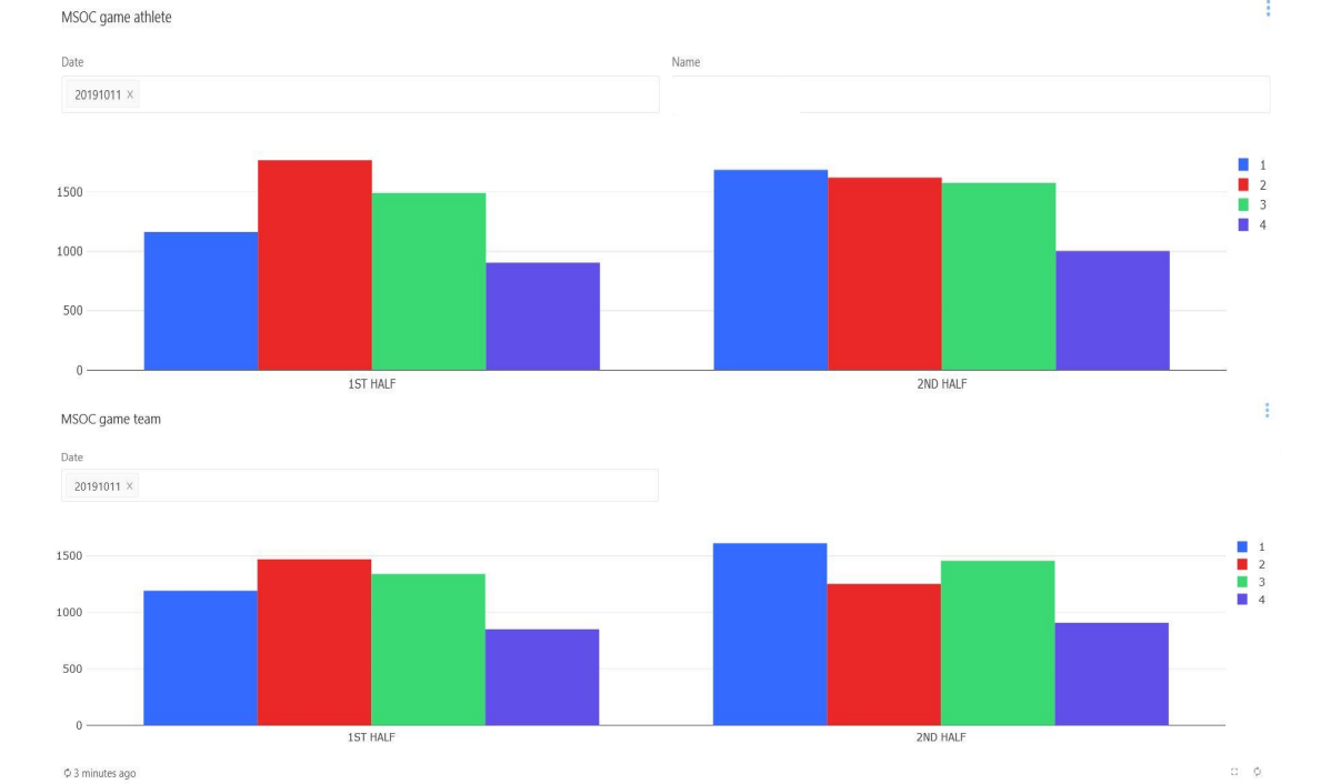
Example: Player Performance by Game
This view of the data enables coaches to evaluate players returning from injury. The coaches are able to compare the player’s performance to the rest of the team. This allows the coaches to effectively manage playing time, ensuring that the player is not too rundown or in need of more recovery time. It also helps determine future training and workload for the athlete.
Next Steps
The next steps going forward with this project are:
- Creating models for data to begin predictive analysis
- Deeper statistical testing
- Developing HPCC Systems machine learning libraries
The project team is currently looking at the connection between the GPS data and how it compares to the subjective data coming in from the questionnaires. The goal is to find any types of relationships or trends that can help predict how the athlete responds to training drills, lifting sessions, or in-game activity. Knowing how the athlete feels after these activities can allow for adjustments for future trainings, ensuring that the athletes are not overtraining or de-training.
End Goal
The end goals for the Athlete 360 program are:
- A 360 view of athlete wellbeing and performance.
- To find the best way to inform process of developing optimized training for athlete’s maximum potential.
- To help sport coaches better understand the demands of practice/competition and make connection between intent of session and real world outcome.
Using data analytics to optimize player training and performance is highly beneficial to sports organizations, coaches and players, trainers, and sports fans across the globe.
Acknowledgement
 A special thank you to Chris Connelly for his phenomenal presentation, “Soccer Analytics: Leveraging Raw GPS Data for Optimizing Player Performance,” at Community Day 2019 and HPCC Systems Tech Talk 29.
Special thanks also goes to Dr. Vincent Freeh, Assistant Director of Undergraduate Programs & Associate Professor at NCSU, for his guidance and leadership on this project, and Raja Sundarrajan, Software Engineer III at LexisNexis Risk Solutions, for his programming expertise.
Watch the full video of Chris Connelly’s presentation at HPCC Systems Tech Talk 29.