Machine Learning and the Forensic Application of Audio Classification

Audio forensics is the field of forensic science relating to the acquisition, analysis, and evaluation of sound recordings. These recordings are normally used as evidence in an official venue. In this blog, we discuss a modern approach to forensic audio analysis, using artificial neural networks, digital signal processing, and big data. 

Muiredach O’Riain, who holds a Bachelor of Science degree in Music with Computing from Goldsmith’s, University of London, introduced his HPCC Systems intern project on “Machine Learning and the Forensic Application of Audio Classification,” at HPCC Systems Tech Talk 30.  The full recording of Muiredach’s Tech Talk is available on YouTube. Muiredach also presented a poster about this project at Community Day 2019.                                                                                                                                                                                                                                                                                                                                                          
The goal of Muiredach’s intern project was to use HPCC Systems to design a reliable classification model that is able to accurately classify an input sound file to the location where it was recorded.  This project demonstrates a proof of concept for this technology, and lays the groundwork for what could be the next step in forensic audio analysis, as well as a new way to gather information through sound.

In this blog, we:

• Discuss Methodology
• Present Results
• Consider Future Applications

Let’s begin by discussing the methodology for this project.

Methodology

The methodology used to construct this model for sound classification is divided into three main parts:

• Data Generation
• Data Processing
• Data Analysis

So, let’s move to the data generation process.

Data Generation

Building an accurate predictive model with a neural network requires a significant amount of high quality data, to “train” the model. This sound classification project required a significant amount of high quality labeled audio files, recorded in different rooms. It would be impractical and time consuming to make thousands of recordings, so this data was generated artificially by using a technique called convolution reverb. 

Convolution Reverb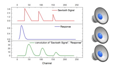

Convolution Reverb is a digital signal processing technique that can be used to simulate the natural reverb of existing spaces digitally. To achieve this, an impulse response (IR), which is typically a quick burst of noise, is recorded in the space to be simulated. This IR is then convolved (combined) with the signal of another sound. The resulting convolution makes it appear as if the other sound was recorded in the room where the original IR was created.   

Convolution Reverb – Impulse Responses

To generate a database of labeled sounds in rooms, two sub databases were created – Impulse Responses of each room and dry audio samples to convolve together and simulate in the spaces.
Impulse Responses were taken from the Aachen Impulse Response (AIR) Database.

Eight different 64-bit, 48000Hz Wav files were extracted and selected to act as IRs and Labels:
IR_1_aula_carolina
IR_2_booth
IR_3_lecture_theatre
IR_4_meeting_room
IR_5_stairway
IR_6_corridor
IR_7_kitchen
IR_8_bathroom

Convolution Reverb – Dry Samples

GNU Wget

GNU Wget is a free, command line program that allows a user to retrieve and download content from websites using HTTP, HTTPS, FTP and FTPS online protocols. By making use of the recursive command, websites and entire domains can be mirrored so that they can be run offline/locally. Alternatively, a Wget can be   used to specify a specific file type to download exclusively, which was the case in this instance.
Dry samples were downloaded from PacDV, a website that hosts a huge database of free non-copyrighted sound files.  A Wget command was used to download all the files on the domain with a ‘.wav’ extension, and the files were then stored on an external hard disk drive.

Batch Convolving and Exporting with Python

With two sub databases of IRs and Dry wav files ready to go, a program was written to quickly generate the dataset that would be used to train the neural net.

Now that we have discussed how the data was generated, let’s move on to the processing of the data.

Data Processing – Cepstrums

The use of 1-D convolution Neural Networks training on the first 3 seconds of each sound file yielded fairly accurate classifications. However, further research showed that the analysis of the cepstrums of signals, rather than the sound itself, produced good results. For this project, when using cepstrums in place of raw audio:

• The accuracy of the predictive models increased dramatically                  
• The size of the training database and time to train dramatically decreased, since a cepstrum of a signal can be represented in a few numbers.

So, what exactly is a cepstrum?

Cepstrums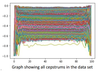

In Digital Signal Processing, a cepstrum is the result of taking the inverse Fourier transform of the logarithm of the estimated frequency spectrum of a signal.
A cepstrum can be seen as information about the rate of change in the different frequency spectrum bands of a signal.

 

Formatting for TensorFlow

The final step of processing data for this model was formatting the dataset to be used effectively with Tensorflow. This involved randomizing the orders of the samples in the data set and formatting the data into a numpy array in an appropriate shape, to be accepted by TensorFlow (TF) as an input for the Neural Net.

Next, we move on to the data analysis portion of this model.

Data Analysis

After generating the dataset, the next step is to analyze the   data and detect patterns to help predict the recording location of a sound file. Artificial neural networks were used to achieve this goal. 

But what is a Neural Network, and how does it train?

Artificial Neural Network

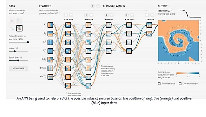
An Artificial Neural Network is a Machine Learning System that can be trained to complete specific tasks by analyzing examples. Learning is achieved by passing data through interconnected layers of nodes (neurons). Each neuron has a weight assigned, which is adjusted as the model is trained on more examples. Using this method, Artificial Neural Networks can automatically detect and generate the identifying characteristics of a dataset.

A good neural net should pull the identifying features from the data during training, and then when it is given an unlabeled file, be able to run it through the system. Based on these factors it detects in the new file, classifying the unlabeled input to the room where it was recorded.

Neural Network

TensorFlow and Optimizing Neural Networks with TensorBoard

TensorFlow and Keras was used to build, design, and run the initial Neural Networks for this project. TensorFlow is a programming library developed by the Google brain team. Keras is an open source Python library for neural networks.

When it comes to building a Neural Network, there are an infinite amount of ways to design and structure your model:

• The number of layers
• The amount of nodes in each layer
• The activation algorithm of each node
• The learning rate 
• Optimizer
• Loss Function

All these factors and more can influence the accuracy of a model, and should be considered when building an Artificial Neural Network.

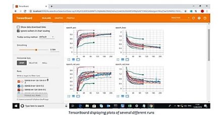
A TensorFlow web application, TensorBoard, was used to visualize and optimize the Neural Network. 

Optimizing Neural Networks with TensorBoard

Using TensorBoard, multiple Neural Networks can be trained. The training process of each Neural

Network run over time can be visualized and compared, to work out which structures perform best.                                                                                                                                                                                      
A series of graphs, can help find the best possible structure.

Results of the Optimization

After using raw .wav data to train the Neural Net, the models with the best results were those that included 1 or more 1D convolutional layers.           
TensorBoard was used to compare these runs with the runs of Artificial Neural Networks that were being trained, and the results showed:

• The cepstral data –Better and faster results were achieved using 3 dense layers of 128 nodes.
• An upside of this is that a dense model also trains far more quickly, taking less than half the time of the model that used convolutional layers.
• The results of these models were very promising and showed a correct classification rate of 85% when classifying between eight rooms, and  90% when classifying between two rooms for the out of sample validation dataset after just 100 epochs.

ECL & HPCC Systems

HPCC Systems was found to be a great resource for this project. To reach its full potential, this project requires the analysis of a lot more data than one computer can handle, and HPCC Systems provides a platform to create models and train them on much larger databases.
Having found a good structure for the Neural Network the models were ported to ECL and the HPCC Systems cluster. 

The Python code used to create the original dataset was modified to output the dataset as a .csv file, to be sprayed to the cluster. 

The following shows “conceptual” code for project.

“Conceptual” Code 

#OPTION('outputLimit',400);
import Python3 as Python;
import HAR.HARDataset as H;
 
outRec := RECORD
    INTEGER one;
    INTEGER two;
END;

result := RECORD
    INTEGER t;
END;    

STREAMED DATASET(outRec) train(STREAMED DATASET(H.Layout) inDS, UNSIGNED otherParam) := EMBED(Python:Activity)
    from numpy import mean
    from numpy import std
    from numpy import array
    from tensorflow.keras.models import Sequential
    from tensorflow.keras.layers import Dense
    from tensorflow.keras.layers import Flatten
    from tensorflow.keras.layers import Dropout
    from tensorflow.keras.layers import LSTM
    from tensorflow.keras.utils import to_categorical
  
    def getOutput(param,r):
            for i in range(len(r)):
                tup = tuple([int(r[i]),int(ytest[i])])
                yield tup
    
    X = []
    y = []
    accuracy = -1
    for rec in inDS:
        l = list(rec)
        y.append(l[-1])
        del l[-1]
        del l[0]
        X.append(l)
    
    X = array(X)
    y = array(y)
    
    y = y.reshape(len(y),1)
    
    split = int(len(X)*0.7)
    Xtrain = X[:split, :]
    Xtest = X[split:, :]
    ytrain = y[:split]
    ytest = y[split:]
    
    ytrain = ytrain.reshape(len(ytrain),1)
    ytest = ytest.reshape(len(ytest),1)
    
    ytrain = to_categorical(ytrain)
    ytest_ = to_categorical(ytest)
    
    Xtrain = Xtrain.reshape((Xtrain.shape[0],8,9))
    Xtest = Xtest.reshape((Xtest.shape[0],8,9))
    
    epochs, batch_size = 15, 64
    n_timesteps, n_features, n_outputs = Xtrain.shape[1], Xtrain.shape[2], ytrain.shape[1]
    model = Sequential()
    model.add(LSTM(50, input_shape=(n_timesteps,n_features)))
    model.add(Dropout(0.5))
    model.add(Dense(50, activation='relu'))
    model.add(Dense(n_outputs, activation='softmax'))
    model.compile(loss='categorical_crossentropy', optimizer='adam', metrics=['accuracy'])
    model.fit(Xtrain, ytrain, epochs=epochs, batch_size=batch_size)
    res = array(model.predict_classes(Xtest, batch_size=batch_size))
    
    return getOutput(2,res)
ENDEMBED;
    
out := train(H.train + H.test,2);
OUTPUT(out);    
//OUTPUT(COUNT(out(t = 0)));
//OUTPUT(COUNT(out))

result check(outRec L,INTEGER C):=TRANSFORM
    SELF.t := IF(L.one = L.two,1,0);
END;

 final := PROJECT(out, check(LEFT,COUNTER));
OUTPUT(final);
OUTPUT(COUNT(final(t=1)));
OUTPUT(COUNT(final));

Uploading, Spraying, and Formatting Data for ECL

With the dataset ready, the next step was uploading the data to the landing zone with ECL Watch and spraying the data to the cluster.

Once uploaded, sprayed the data was sprayed using a DELIMITED spray. Once the data was on the cluster, it was ready to work within the ECL IDE.

A record layout was written for the database, and the dataset was exported in that format, ready to be used with Generalized Neural Networks (GNN) to create a Neural Net

GNN & Technical Difficulties

GNN is a ‘Generalized Neural Networks’ bundle for HPCC Systems ECL IDE, created by Roger Dev, that provides a generalized ECL interface to Keras over Tensorflow. The Generalized Neural Networks (GNN) bundle: 

• Provides Keras / Tensorflow operations parallelized over an HPCC Systems Cluster.
• Creates models on each HPCC Systems node, and allows for training, evaluation, and predictions in a distributed fashion across the HPCC Systems cluster.

When this project was in progress, GNN was not fully functional. As such, the model was not able to be run successfully on the HPCC Systems platform without errors. 

The GNN bundle is now functional and available for general use. For more information on the GNN bundle, see the blog post “Analyze images, videos, time-series and more with the Generalized Neural Network bundle (GNN),” by Roger Dev. This informative blog post gives a detailed explanation of the GNN bundle, and provides instructions how to download and use the software.

Final Conclusions

Machine Learning and the forensic application of audio classification is a project focused on the classification of sounds for forensic purpose. The results of this study have been extremely promising in helping to define a link between the spectral properties of a room and the classification of sounds recorded in said room. This research provided compelling evidence for the ability of artificial Neural Nets to define and utilize these connections to create a reliable classification model.

Limitations

As with any model, there are certain limitations that should be explored, and how they affect the results of this particular study should be analyzed. For example, the use of generated data rather than original recordings means that all the sounds are “recorded” from the same position within the room, with the same recording equipment. In addition, the model can currently only differentiate between sounds in 8 different rooms.
In order to create an ideal system that could identify more about the size and space of any room, this model would need to train on a lot more data.

Final Thoughts

There is still a long way to go before this technology could have any real world applications in the field of forensic audio, but a strong foundation has been laid. The results of this project can definitely be seen as an encouraging starting point for future work on this topic.

About Muriedach O’Riain

Muiredach holds a Bachelor of Science degree in Music with Computing from Goldsmith’s, University of London. During his degree, he designed a smart sampler instrument to use sound recognition and data mining techniques, along with AI, to match an input sound to the closest corresponding sound from a bank of samples in real time. This meant he could take, for example, a beat boxer and match each ‘hit’ to the corresponding sound from the sample bank, converting the human voice into an electronic drum machine. Muiredach also designed a C++ and DSP music application to combine physical modeling synthesis with an intuitive, interactive visual interface to create interesting soundscapes.