Learning Trees — A guide to Decision Tree based Machine Learning

Introduction

Today, there are three major classes of Supervised Machine Learning algorithm:

• Linear Models
• Neural Network Models
• Decision Tree Models

In this article, we take a dive into the world of Decision Tree Models, which we refer to as Learning Trees.  We explore the mechanisms and the science behind the various Decision Tree methods.  Additionally, we provide an overview of HPCC’s free LearningTrees Bundle that provides efficient, parallelized implementations of  these methods.

This article assumes a general knowledge of Machine Learning and its terminology.  For an introduction to Machine Learning, see: Machine Learning Demystified.  For a tutorial on installing and using the Learning Trees Bundle, as well as other HPCC Machine Learning methods, see: Using HPCC Machine Learning.

Learning Trees

Decision-tree based Machine Learning algorithms (Learning Trees) have been among the most successful algorithms both in competitions and production usage.  A variety of such algorithms exist and go by names such as CART, C4.5, ID3, Random Forest, Gradient Boosted Trees, Isolation Trees,  and more.  Each of these algorithms has different characteristics, benefits, and limitations, but are all based on a common model — a Decision Tree.  Decision Tree ML methods share a common set of benefits and disadvantages vis-a-vis other ML methods.

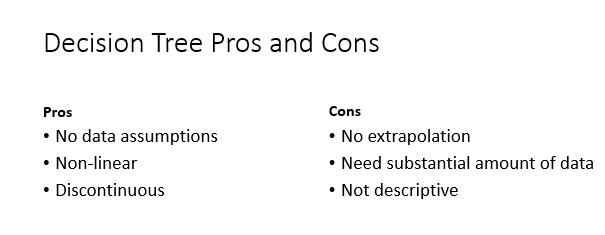
Figure 1 lists the major advantages and disadvantages of Decision Tree based methods.  Their flexibility in learning provides their key advantage.  There are no assumptions as to the nature of the data or the relationships between features as are common in many other algorithms.  Learning Trees can handle very complex data with unknown / unspecified data relationships in stride.  On the other hand, a fairly large set of data is typically required in order to get strong predictions.  This is because there is no extrapolation of the data relationships.  If the training data doesn’t cover the full range of values and relationships, then there will be blind spots in the predictions which may result in some large errors.  Contrast this with a linear model, where a few points can potentially yield a reasonable model that can make its predictions over a wide space — provided that the phenomenon being modeled fits the assumptions of the model.  While Learning Tree methods are considered interpretable (compared to some other methods), complex models are still challenging to comprehend.

Decision Tree Overview

Decision Trees have been used, at least, since the 1930’s as a way to structure knowledge using a cascading set of rules.  They are conceptually simple and reasonably easy to understand and interpret.

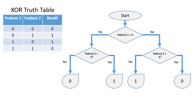
Figure 2 illustrates a simple binary decision tree depicting an Exclusive-OR (XOR) operation.  If the first feature (i.e. variable) is 0, we will take the left branch, which checks the second feature.  If the second feature was 0, the tree will output 0 as the result.  If the second feature was 1, then the result will be 1.  On the right branch, where feature 1 had a value of 1, it then asks the same question about feature 2.  In this case, if feature 2 was 0, the result is 1, while if 1, the result is zero.  Note that we could have built the tree differently by asking about feature 2 first.  There are typically, many ways to organize a tree for any complex problem.

Each node (branch) in the tree asks a question, which when answered leads to one of two other questions.  Each of those questions lead to other questions.  At the bottom of the tree, are the leafs.  The leaf represents a particular outcome, based on the answers given to each of the hierarchical questions.  Given a set of answers, the tree will always present an outcome.  The outcome could be, for example the answer to a complex problem such as identification of a species, the proper setting for an instrument,  the diagnosis of an illness, or a recommended action.

Geometrically, each question separates the points orthogonally — perpendicular to a given feature axis. This can be visualized as horizontal or vertical lines that subdivide the space into finer and finer squares at whatever resolution is necessary to separate the training points.  Of course, in a real work problem with many features (i.e. dimensions), we are using orthogonal hyper-planes to segment the space into finer and finer hyper-cubes. 

Decision trees were historically constructed by hand as a way of embedding expert knowledge in a form that was easy to interpret.  But in the early 1980’s, a series of papers described a way to automatically construct decision trees based on collected data (observations) and desired outcomes for each observation (labels).  Based on a collection of labeled observations, a tree could be algorithmically built that would be able to choose the correct outcome (label) for each observation based on questions about the observed features.  If a diverse enough set of labeled data was presented during construction of the tree, then the tree would be able to determine the outcome (label) for any new observation.  This was an early form of machine learning that would work well for almost any deterministic phenomenon for which enough labeled data could be obtained.  Imagine a well-defined set of symptoms that were observed in a set of patients.  Imagine further, that each patient was diagnosed by an expert physician and assigned a disease.  If one were to ask the physician what were the rules on which she based her diagnosis, she would probably profess a long list of symptoms associated with each disease, as well as some “rules-of-thumb” and exceptions to those rules.  The physician would not likely be able to express a coherent road-map that would let a non-practitioner make a useful diagnosis.  But given the symptoms and the physician’s diagnoses, a simple decision-tree learning algorithm can determine the questions to ask in order to assign diagnoses.  This effectively reverse-engineers the physicians expertise and encodes it into a decision tree.

This works quite well as long as the problem is deterministic — that is, the same features always yield the same results, and there is sufficient training data.  If the problem is stochastic — embodies randomness within the data or outcomes — a decision tree will not likely generalize well.

Let’s take a step back and look into the concept of generalization.

It is important to understand the nature of Population versus Sample.  The training data for a ML model is almost always a small sample of the target population as illustrated by Figure 2 below.

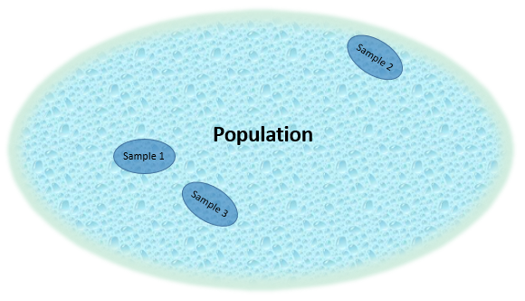
Imagine that we are trying to determine the age of a tree based on easily measurable features such as girth, height, annual rainfall, and elevation.  The population, representing the target of our endeavor, might be: any tree, of any species, anywhere on earth, past, present or future.  Compare that to our training data which is, at best, a few thousand samples of a few dozen species in a few hundred locations.  This is, of course, a minuscule proportion of the target population, which is effectively unbounded.  A single decision tree will, in most cases, correctly categorize every single point in the training data.  Since it has learned to separate every point in our extensive training set, shouldn’t we expect that it will work quite well against another sample of the population?  The short answer is No.  There are several reasons for this:

• Underfitting — If our sample covers only a tiny percentage of our population, it is very likely that a second sample would represent species, locations, and environments that we never encountered in our sample.  One way to address this issue is to refine our definition of the population.  For example:  A limited set of species in a limited geography.
• Non-separability — What happens when we have two trees, of two very different ages that have every other feature in common?  We can choose the most commonly occurring age with those feature values, but that will certainly cause errors since that choice will cover up the other possibilities.  Alternatively, we could average the results, but this will also cause errors.  Generally, if this is a common occurrence, it is a sign that there may be some missing features that might provide better discrimination.
• Overfitting — Probably the most common cause of problems.  It occurs when an ML algorithm uses noise within the sample to separate points.  Any sample of a population will contain noise.  If I flip a coin three times, I may get three heads in a row.  If I flip a coin a hundred times, I may get 60 tails.  If I use any small sample, I will be subject to “random perversity”. In real-world scenarios, such noise may be the result of randomness within the population, errors during data collection, or errors during data curation.  Utilizing this noise in the decision process creates a model that is more complex than is warranted, and can result in poor prediction against other samples from the population.  Overfitting is difficult (if not impossible) to detect during the training process, because we are after all, have no view into the population except through the window of the training data.  It is tempting to think that spurious correlations in the data can be eliminated with a large training set, but as the learning process descends through the tree toward the leafs, fewer and fewer points are being split at each node.  Therefore, the data at those levels is susceptible to frequent spurious correlations — if two features can split the data points effectively, there’s no way to tell which feature is discriminatory, and which is coincidental.

A key value for any ML algorithm is the extent to which its model Generalizes to population samples outside of the training sample.

In the early 1980’s, several researchers noticed something surprising.  If we use multiple learning techniques, and average the results from each, it can dramatically improve the accuracy of predictions against the general population.  In the 1990’s, researchers applied this same approach to a “forest” of diverse decision trees and found that it almost entirely eliminated the problem of overfitting. 

Random Forest

This technique was named “Random Forest”, and was found to be one of the most accurate and easily used forms of machine learning.

In a Random Forest, a series of decision trees are grown, with some randomness added to the growth process to ensure that each tree used a different decision process to separate the points.  Then, for each new data point, all of the trees are queried for their prediction.  These individual predictions are aggregated to form the final prediction.  If the goal of the forest is to choose one of several classes (i.e. a Classification Forest), then aggregation is done by voting:  the class predicted by the largest number of trees becomes the final prediction.  If the goal is to predict a numeric value (such as age), then we have a Regression Forest, which forms a final prediction by averaging the predictions of the various trees [1].

The key to the success of this approach is diversity.  Clearly, if we grew a forest of trees without added randomness, they would all make the same prediction.  Nothing would be gained by aggregation of such a forest.  Random Forests use several methods to introduce the requisite randomness:

• Resampling — Each tree is grown on a subset of the training points.  This is done by choosing points randomly from the training set.  If there are a thousand training points, then each tree will randomly choose a thousand points from the training set.  Some of those will be duplicates, and some of the points will not be chosen by that tree.  In effect, each tree will be trained on about two thirds of the points in the training set.
• Feature Restriction — At each step of tree building, a subset of the features are randomly chosen, and the best feature and split point is chosen from that reduced set of features.  This forces different decisions to be used early on in the growth of a tree, which causes a very different decision process.

One of the wonderful characteristics of Random Forest is that there are very few parameters to tweak, and the choice of those parameters generally have very little bearing on the accuracy of the results.  Good results can usually be achieved using the default parameters, making it one of the most user-friendly ML algorithms.

Another great characteristic is that Random Forest can deal with large numbers of features.  It is not uncommon to use RFs with thousands of features.

Finally, Random Forests are easily parallelized and are, therefore, an ideal algorithm for use on HPCC Systems clusters.

Boosting

In the late 1980’s, another approach was being developed for improving the accuracy of Machine Learning methods.  Researchers wanted to know if a weak learning algorithm could be made strong by focusing the algorithm on successively more difficult distinctions.  This approach was called “Boosting”.  The weak learner concept has been codified as PAC (Probably Approximately Correct) Learners.  In Boosting, a PAC learner attempts to predict the result, and the items it got wrong are emphasized and sent to another PAC learner.  This process is repeated for some number of iterations and the results of all the learners are aggregated.  This ideally results in the early learners solving the easy-to-distinguish cases, while the later learners become focused on the more difficult cases.  The theory was that the aggregate should be more accurate than any of the PAC learners, and perhaps compete with stronger learners.  The theory was proven correct, and Boosting has produced some very powerful learning systems.  In the late 1990’s, researchers looked at shallow trees (i.e. trees with only a few levels) as PAC learners and created a number of very successful “Boosted Tree” algorithms.  In the early 2000’s, several methods were generalized as Gradient Boosted Trees (GBTs).  GBTs form a linear hierarchy of trees, where each subsequent tree attempts to correct the errors of the previous tree, and the results are added together to form the prediction.  These GBTs have proven to be very good at squeezing information out of the training data since they iteratively work on the more difficult distinctions.  They also tend to generalize quite well.

While GBTs can, in some cases, produce better accuracy than Random Forest, they have a few disadvantages:

• Ease of Use — There are a number of interacting parameters that have to be calibrated (i.e. regularized) in order to achieve near-optimal results.
• Sequential Operation — Boosting is inherently sequential — the results from one Tree are needed before training the next tree.  This makes it difficult to take advantage of a parallelized architecture like HPCC Systems.

If we peel back the layers and see what’s going on with GBTs, we see two distinct activities at work simultaneously:

• Boosting — Focusing the decision process on harder and harder distinctions.
• Generalization — Reducing the effect of “Random Perversity” on the decision process.

If enough Boosting iterations are done, it has the side effect of Generalization.  That is because all of the boosted trees are aggregated to produce the result.  Diversity of trees is automatically guaranteed by the fact that each successive tree is trained to the errors of the previous trees.  They are therefore built on different training data and will not likely repeat the same decision process.

We wondered what would happen if we separated these two activities.  We hypothesized that fewer boosting iterations would be necessary if we pre-generalized each layer of the boosting hierarchy.  This would improve the performance on a parallelized cluster architecture like HPCC.

Boosted Forests

So we tried using a Random Forest as the learner, rather than a shallow tree.  We restricted the depth of the trees in the Forests to create a weak learner (as was done for GBT) and found that, indeed, fewer iterations were needed to achieve the same accuracy.  We further noted that it mattered little whether we used shallow trees (i.e. weak learners) or fully developed trees (i.e. strong learners).  We found that most of the tuning necessary to get good results using GBT was needed in order to properly generalize, and very few boosting iterations were actually needed to achieve optimal results.  We dubbed this approach Boosted Forests (BFs), and with further study found that these BFs work very well and significantly outperform Random Forests for regression.  Furthermore, BFs provide for an automatic stop criterion that stop iterating once essentially all of the variance in the training data has been accomodated by the model.  With the stopping criteria, we have an algorithm as easy to use as Random Forest, but with accuracy comparable to the best parameterization of GBTs.  We have found that BFs can in five iterations produce better results than GBTs with hundreds of iterations.  Plus they are far more parallelizable than GBTs.  Generalization can be parallelized while boosting cannot.  By separating the two activities, we achieve both generalization and boosting in fewer iterations.

Curiously, we were not able to achieve similar results with classification.  We tried four different boosting methods to improve upon the accuracy of Classification Forests, and none was able to consistently exceed that of the Classification Forest.  It should be noted that GBTs have not been shown to improve on the accuracy of Classification Forests either.

We don’t quite understand why this is so, but we believe it has to do with: a) the fact that Classification Forests directly process rules similar to the natural rules that govern the classification while Regression Forests use rules of separation to approximate continuous processes and b) that continuous regression results can be tweaked (via boosting) to nudge the results (average of all trees) to a closer match to the data, while classification results are either right or wrong with no opportunity for nudging.  Another way to look at it is that Classification Forests produce results that are very close to a theoretical accuracy limit, Regression Forests produce results that can still be improved upon.  We hope to further research this and understand this process better.

Boosted Forests are not without weaknesses, however:

• Performance — A BF naturally takes more resources than a Random Forest.  For example, if it takes five levels of boosting to achieve optimal results, than it will take around 5 times longer to run than an equivalent Random Forest.  It will also take somewhat longer to make predictions than a Random Forest.  On an HPCC Cluster of sufficient size, a BF may run faster than a GBT.  This is because the Random Forest component is parallelized, and fewer iterations are needed compared to GBT.
• Standardization — Boosted Forests are not well established in the literature and may not, therefore, be accepted in some applications.

The LearningTrees Bundle

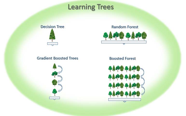
The LearningTrees Bundle provides an efficient, scalable implementation of Learning Tree methods.  It currently provides Decision Trees, Random Forest, Gradient Boosted Trees and Boosted Forest algorithms.

LearningTrees has additional capabilities that add to its power and ease-of-use:

• Features can be any type of numeric data:
  • Real values
  • Integers
  • Binary
  • Categorical
• Output can be categorical (Classification Forest) or real-valued (Regression Forest).  Multinomial classification is supported directly.
• Myriad Interface — Multiple separate forests can be grown at once, and produce a composite model in parallel.  This can further improve the performance on an HPCC Cluster.
• Accuracy Assessment — Produces a range of statistics regarding the accuracy of the model given a set of test data.
• Feature Importance — Analyses the importance of each feature in the decision process.
• Decision Distance — Provides insight into the similarity of different data points in a multi-dimensional decision space.
• Uniqueness Factor — Indicates how isolated a given data point is relative to other points in decision space.

In LearningTrees a Decision Tree is implemented as a Random Forest with number-of-trees set to 1, and a GBT is a Boosted Forest with forest-size set to 1.

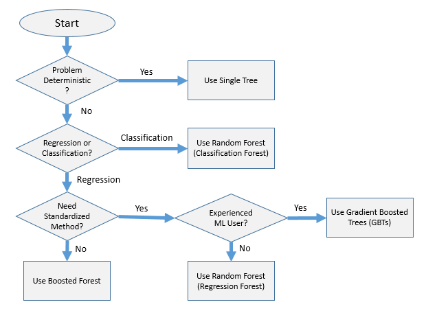
Algorithm Choice

So, which algorithm should you choose?  The flowchart below should be used to assist with your decision.

In Closing

Tree-based algorithms are probably the most powerful and easy-to-use algorithms in the Machine Learning arsenal.  If your data is numeric, there is a reasonable amount of data, and the goal is Prediction rather than explanation, it is hard to do better than Learning Trees.