An Investigation into Time Series Analysis

Time series forecasting is an important statistical tool for predicting future events, needs, trends, etc., and can be applied to a variety of data sources. Jeremy Meier and David Noh, recent graduates of Clemson University’s Computer Science program, spoke at HPCC Systems Tech Talk episode 23 about the basic principles and components of time series forecasting using modern machine learning methods. This blog gives insight into their semester-long project, which focused on time series analysis and Forecasting using financial datasets. 

The project team worked closely with datasets that had approximately 16,000 total observations, recording dates and balances from the financial data. The focus was on individual accounts with a size of around 400 observations. The initial goal was to compare statistical metrics and techniques used commonly in time series analysis on the given datasets. 

Two major industry standard methods were used to analyze the datasets, with the goal of predicting future balances in the dataset and identifying any anomalies or misbehavior in the data, for the purpose of providing business value. 

In this blog we:

• Provide deeper insight into time series analysis and time series forecasting.
• Discuss various techniques for analyzing and modeling time series data. 

Let’s begin by defining time series analysis and Forecasting.

Time Series Analysis and Forecasting

Time series analysis comprises methods for analyzing time series data, in order to extract meaningful statistics and other characteristics of the data. Time series forecasting is the use of a model to predict future values based on previously observed values.

What is a Time Series?

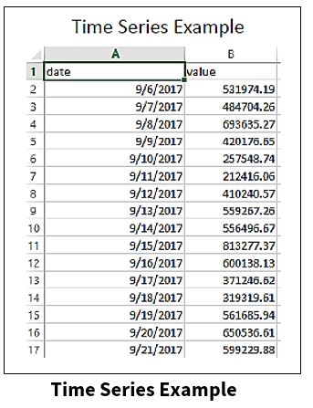
A time series is a series of data points that are measured in regular or semi-regular intervals. 

The chart below shows a time series dataset. This data was collected and measured at different time intervals. 

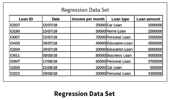
The regression dataset below has multiple predictors, which includes the date, income per month, loan type, and loan amount. This is a big distinction between time series and other datasets, especially when it comes to analyzing and forecasting, and the different approaches that come along with those models. 

Continuing on with the definition of time series, a time series is:

• A series of data points indexed in time order. 
• A sequence taken at successive and equally-spaced points in time.

Some real-world examples of time series are recording the heights of the ocean tides, the number of sunspots, or the daily closing value of the Dow. 

There are four components generally associated with time series:

(1) Seasonal variations that repeat over a specific period such as a day, week, month, season, etc. 

(2) Trend variations that move up or down in a reasonably predictable pattern. 

(3) Cyclical variations that correspond with business or economic ‘boom-bust’ cycles or follow their own peculiar cycles.

(4) Random variations that do not fall under any of the above three classifications.

Generally, time series have some sort of “seasonality” or “trend.”

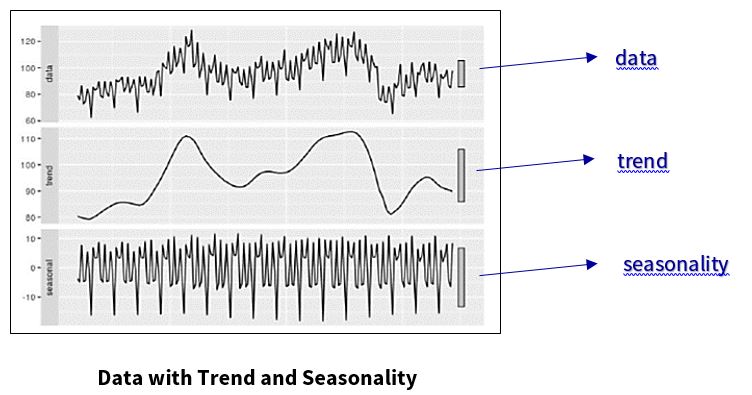
• Trend – A component of a time series that shows the overall movement in the series, ignoring the seasonality and any small random fluctuations.
• Seasonality – Presence of variations that occur at specific regular intervals.

In the example below, the “data” is located at the top portion of the chart and the “trend” is located in the middle. For “trend,” the small random fluctuations have been removed from the original data. “Seasonality” is shown at the bottom of the chart. In the portion of the chart that shows “seasonality,” the “trend” has been removed, and shows variations at specific regular intervals.  

Stationarity is a vital assumption for time series modeling and forecasting. Let’s take a look at stationarity and why it is so important.

Why is Stationarity important?

Stationarity is a common assumption in many time series techniques. A stationary time series is one whose statistical properties such as mean, variance, and autocorrelation are all constant over time. 

• Time series with trends or seasonality are not stationary.

Most Statistical modeling methods assume or require the time series to be stationary in order to be effective.

• Stationary time series are easier to predict when they are stationary: one simply predicts that statistical properties will be the same in the future as they have been in the past.

To further explain the importance of stationary data, consider this illustration. If a time series is consistently increasing over time, and the sample mean and variance grows with the sample, this will lead to a constant underestimation of the mean and variance in future periods, causing issues with many models used in time series analysis and forecasting. 

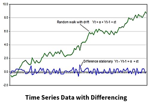
The chart below shows a plot of time series data. The original data is shown in green. The data shown in blue is the plot of the time series data after “differencing.” Differencing is a method of making time series data stationary. After differencing, the variance and covariance are constant. 

How do I know if my time series is stationary?

To determine if time series data is stationary:

• First, plot the time series and evaluate the variability of the time series.
• Review the summary statistics for your data for seasons or random partitions and check for obvious or significant differences. 

Split your time series into two (or more) partitions and compare the mean and variance of each group.                       

• Statistical tests can be used to check if the expectations of stationarity are met or have been violated.

The Augmented Dickey-Fuller test allows the user a high degree of certainty that their data is stationary. However, it is a statistical approach, and does not fully “guarantee” that the data is stationary.

How do I make my time series stationary?

Making your data set stationary can usually be accomplished through the use of mathematical transformations.

Two types of mathematical transformations are:

Differencing

• The “lag difference” takes the difference between consecutive observations.

Example: 

Original time series: X1, X2, X3,………..Xn

Time series with difference of degree 1: (X2 -X1, X3 -X2, X4 -X3,…….Xn -X(n-1)

• The process of differencing can be repeated more than once, and is usually repeated until all temporal dependents have been removed from the dataset. 
• The number of times that differencing is performed is called the “differencing order.” 

Transformation

• With this approach, the user takes the log, square-root, or the cube root, etc. of a dataset, in order to make it stationary.
• The data series can be “untransformed” by reversing the mathematical transformation. 

Now that we’ve discussed how to make time series data stationary, let’s move on to time series forecasting.

What is Time Series Forecasting?

Time series forecasting involves taking models fit on historical data and using them to predict future observations. 

In time series forecasting:

• Components, such as trend and seasonality, are often the most effective ways to make predictions about future values, but not always. Some models require the removal of  trends and seasonality. 
• The future is completely unavailable and must only be estimated from what has already happened.
• Performance is determined by how well a model forecasts the future.

With this in mind, let’s take a closer look at the dataset used for this project. 

The Project Dataset

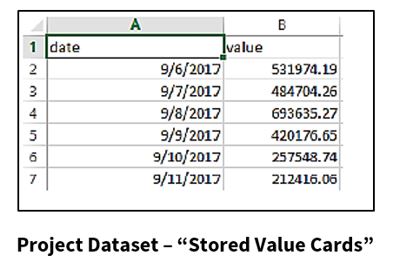
• The name of the dataset used for the project is “Stored Value Cards.”
• The dataset has around 16,000 total observations with around 115 accounts.
• It has two columns of data, making it a time series: a date, taken at intervals, and a value on each of those dates. 
• The opening balance values range from 0 to $10,000,000.00, which represent the balance in the account.

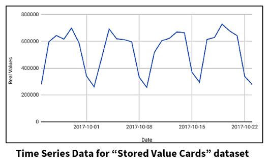
The graph below shows time series data, taken over a period of one month, for the “Stored Value Cards” dataset. This graph will be used throughout the remainder of this blog when referring to forecasting models.

Next, we will take a look at a forecasting method called the “Simple/Naïve Method.”

What is the Simple/Naive Method?

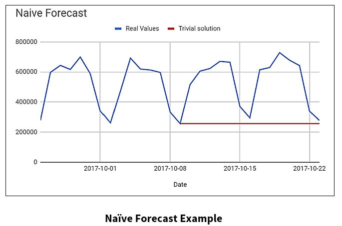
The Simple/Naïve Method is a forecasting technique, where the value of a new data point is predicted to be equal to the previous data point. The result is a flat line, since all new values take the previous values.

Observations for this project:

• The Naïve (Trivial) solution proved to be a powerful tool for predicting one data value in advance.
• The Trivial solution begins to have trouble for multiple-day forecasts.

Let’s take a look at the application of the Naïve method. In the chart below, the blue line is the actual data, and the red line is the Naïve solution. 

The Naïve Forecast Method was used at a bad place in the data to demonstrate its weaknesses. 

We will now look into some more advanced methods for forecasting. 

The Simple/Moving Average Method?

The Simple Average Method is a forecasting technique, in which the next value is taken as the average of all the previous values. 

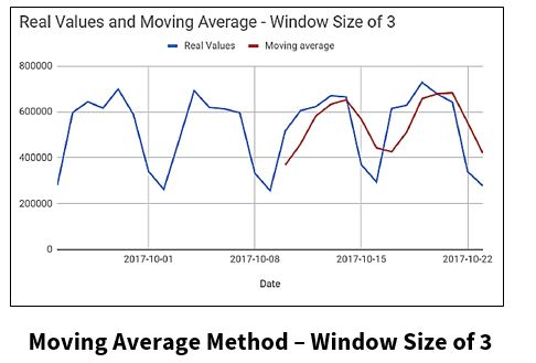
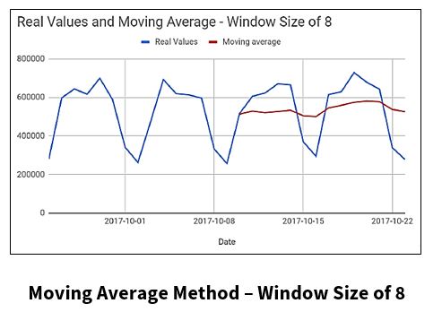
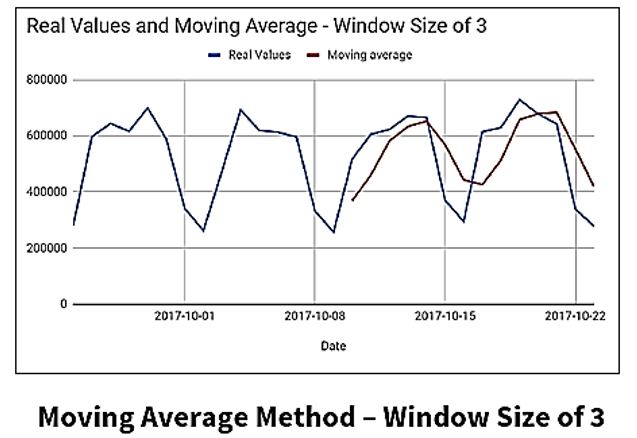
For the Moving Average Method, the next value is derived from the averages of successive segments (values in a given window), not the entire set. The window size can be set by the user.

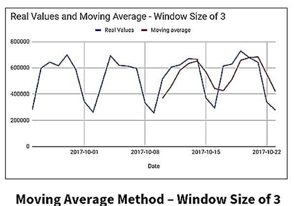
• The window size (lag) can have big effect on the forecasting accuracy of the Moving Average Method. So, when using this method for forecasting on a dataset, some fine-tuning will need to be applied, as shown in the charts below. 

Let’s continue on with some additional time series forecasting techniques.

The ARIMA Model

The ARIMA (AutoRegressive Integrated Moving Average) model is a popular technique used for time series forecasting. This statistical analysis model uses time series data to either better understand the data set, or to predict future trends

The three major parameters of ARIMA are:

Autoregression 

• Model shows a changing variable that regresses on its own lagged or prior values

Integrated

• Represents the differencing of raw observations to allow for the time series to become stationary

Moving Average

• Incorporates the dependency between an observation and a residual error from a moving average model applied to lagged observations.

ARIMA works on two assumptions:

• The data is stationary
• The data provided has input and is a single-variable series. 

Although ARIMA is a powerful model for forecasting time series, the effort to prepare the data and fine-tune the parameters is very time-consuming. Because ARIMA works under the assumption that the data is stationary, one would need to manually make the data stationary in order to find the parameters or the order of differencing.

Auto ARIMA eliminates the need to “stationarize” time series data when using the ARIMA model.

What is Auto ARIMA?

• Auto ARIMA is a model that chooses the parameters and makes the data stationary.

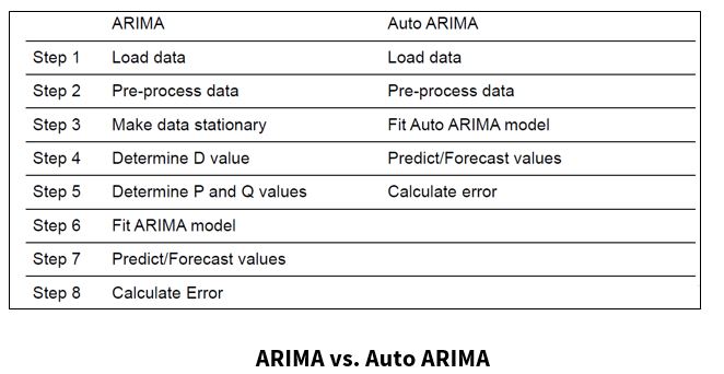
The chart below shows that Auto ARIMA takes out steps one thru six from the ARIMA model steps.

Auto ARIMA does a parameter sweep, and calculates the accuracy for each set of parameters. 

With these accuracy metrics, Auto ARIMA takes the most accurate model and saves it.

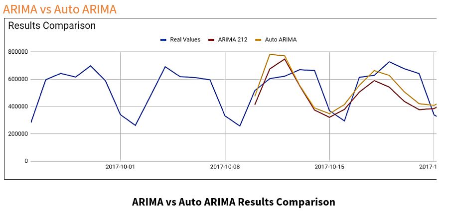
Here we have results from the ARIMA and Auto ARIMA models predictions on the “Stored Value Cards” dataset used for this project. They both seem similar, but Auto ARIMA hugs the second curve of the actual data closer, and is almost identical to the first curve of the ARIMA model’s results, which makes the Auto ARIMA model more accurate than the manually-tuned ARIMA model. 

ARIMA vs Auto ARIMA

Auto ARIMA saves time and effort when parameters have not been tuned for the ARIMA model, but takes more computational time.  

Finally, let’s discuss some modern techniques for time series analysis. 

What are some modern techniques for time series analysis?

Facebook Prophet:

• is an open-source forecasting tool.
• is a procedure for forecasting time series data based on an additive model where non-linear trends are fit with yearly, weekly, and daily seasonality, plus holiday effects. 
• works best with time series that have strong seasonal effects and several seasons of historical data. 
• is robust to missing data and shifts in the trend, and typically handles outliers well.

Random Forest:

• is a supervised learning algorithm.
• can be used for both classification and regression problems.
• normally used in multi-variate datasets, comparatively to the normal time series analysis models that use univariate datasets.

This chart displays results from the Auto ARIMA and Random Forest Models for the “Stored Value Cards” dataset.

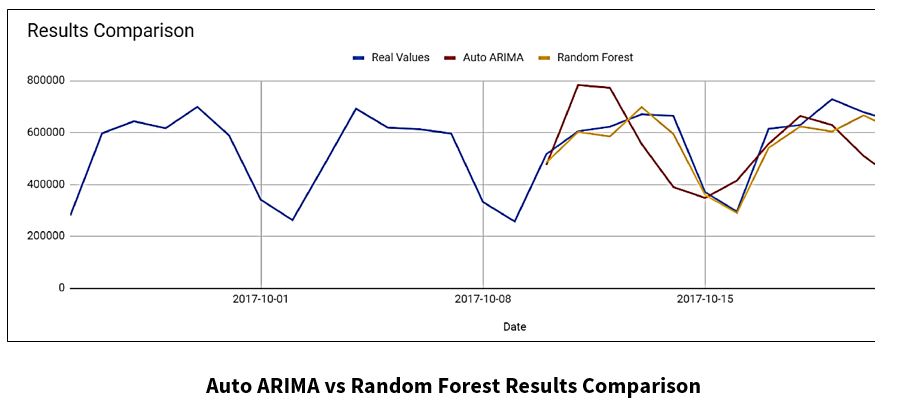
The Random Forest Model fits the “Real Values” curve more accurately than the Auto ARIMA Model.

Although the Random Forest model works better for this dataset, the optimal technique or model can change, based on the dataset.

Summary

Time series forecasting can be used in a variety of areas, such as business, healthcare, technology, politics, etc. The objective of this project was to add business value. In business, time series analysis and forecasting are a vital part of modern organizational management. Forecasting is an important part of business planning, and planning is the backbone of effective operations within an organization. Forecasts are critical for short-term and long-term business decisions, and can contribute to the success or demise of an organization.  

The goal of this project was to compare statistical metrics and techniques typically used in time series analysis on a financial dataset. For this project, several time series forecasting models were applied. The results are the following:

• The Simple/Naïve Method is a powerful tool for predicting one data value in advance, but had trouble for multiple-day forecasts.
• For the Moving Average Method, the window size (lag) affected the forecasting accuracy. So, when using this method for forecasting on a dataset, some fine-tuning will need to be applied to the data. 
• ARIMA is a powerful model for forecasting time series, but because it works under the assumption that the data is stationary, one would need to manually make the data stationary in order to find the parameters or the order of differencing. This is very time consuming. 
• Auto ARIMA eliminates the need to “stationarize” time series data when using the ARIMA model, which saves time and effort on the front end. But, Auto ARIMA takes more computational time. 
• The Random Forest Model was the best time series forecasting model for the “Stored Value Cards” dataset. It fit the “Real Values” curve better than any other model. 

**Please note that although the Random Forest model worked best for this dataset, the optimal technique or model can change, based on the dataset.

About Jeremy Meier and David Noh

Jeremy Meier and David Noh are graduates of Clemson University’s Computer Science program and have begun their professional careers. Jeremy Meier’s research at Clemson University focused on time series analysis. He also worked with HPCC Systems in the development of text analysis libraries. His interests include bioengineering and animation. During his time at Clemson University, David Noh’s research included time series analysis and machine learning algorithms. His interests include machine learning algorithms and high-performance computing. 

Acknowledgments

A special thank you to Jeremy and David for their phenomenal presentation, “An Investigation into Time Series Analysis.” I would also like to thank Dr. Amy Apon (Professor and Chair – Division of Computer Science School of Computing at Clemson University), for her review and input for this blog. And last, but not least, a special acknowledgment goes to Roger Dev (Sr. Architect at LexisNexis Risk Solutions) for his mentorship. 

Listen to the full recording of Jeremy Meier and David Noh speaking about “An Investigation into Time Series Analysis” at our HPCC Systems Tech Talk 23 webcast.