Random Fourier Features accelerated Gaussian Process Regressor

Gaussian process regression is a powerful machine learning method to solve non-linear regression problems. However, because of the intensive computation, Gaussian process regression is not suitable for large-scale machine learning problems. Fortunately, researchers developed approximation methods to get a solution arbitrarily close as the original Gaussian process more rapidly and with better scaling. In this post, a Random Fourier Features accelerated Gaussian process regressor will be introduced. It’s implemented in HPCC Systems to utilize its highly parallelized computing environment.

If you are new to machine learning or interested in supervised learning, the blog Machine Learning Demystified is a great resource. It reviews the basic concepts, terminology of Machine Learning and how to utilize supervised machine learning.If you are interested in unsupervised learning and KMeans algorithm, the blog Automatically Cluster your Data with Massively Scalable K-Means is a good starter. If you are interested in the details of Myriad Interface, you may want to start from this article. This article also assumes that you have at least some basic ECL programming skills, which you can get by reading our ECL documentation or  taking an online training course by clicking here.

As we all know, linear regression is a very popular and basic machine learning model to solve regression problems. In linear regression, we assume the input data has a linear shape with additional noise:

Where the noise term follows a normal distribution:

However, in the real world, only few relations are truly linear, and we need to find a way to solve general non-linear problems.

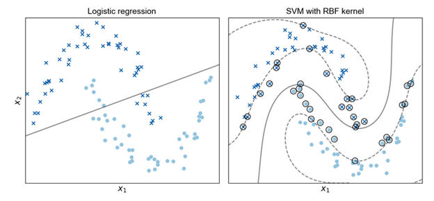
Here kernel methods come to play. Kernel methods defines a function that maps the input data onto a feature space which transforming the inputs with a non-linear function. This transformation results in a n-dimensional vector of numeric features in the feature space. With kernel method, we can apply the familiar linear functions on the transformed features again. Figure 1 shows how kernel method help solve non-linear problems. In the left figure of Figure 1, apparently the linear regression cannot fit the data well and reflect the true relations between x1 and x2. Instead in the right figure of Figure 1, after transforming the input space onto feature space using Radial Basis Function(RBF) kernel, a linear function can model the relations much better than the left figure.

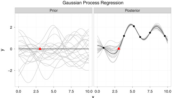
A Gaussian process is a linear function applied on the space transformed via kernel function to solve non-linear problems. Figure 2 shows one example of Gaussian process regression to fit a very small dataset. As we can see from the left figure of Figure 2,  it’s a distribution over functions instead of scalars in linear regression. The average sum of all these functions is optimal estimation of each data point as shown in the right figure of Figure 2. In a simple form, Gaussian process regression can be written as following:

Which looks very similar to linear regression. However, here the f(x) is also a random variable which has its own particular distribution, and it can be defined as following:

Here m(x) is the mean function that take average of all functions in the distribution at an observation point. k(.) is the kernel function of the Gaussian process. There are different kernel functions, and one popular and powerful kernel is the Radial Basis Function (RBF) kernel, also known as a Gaussian kernel:

All these equations are not the central piece of this article if you feel stressed by any means. The key point starts from here: the computation to inference the kernel function is very intensive and grows cubically as the number of data points grows. The computation of prediction or the posterior via a Gaussian Process is even more intensive. Such intensive computation cost hinders the use of Gaussian Process regression for large scale applications.

One adjustment to approach the scalability of Gaussian process regression is to apply Random Fourier Features on the feature space.  It’s first introduced by Rahimi & Recht [1] in 2007 as an approach to approximate and scale up kernel methods. In a nutshell, instead of working the inner project of N by N kernel matrix (N is the number of samples), the authors find a randomized map to project and approximate the feature space with a fewer features. This reduce the computation cost for solving a Gaussian process. Why it’s a good idea and its theoretical proof is out of the scope of this article, but you can find more details from here. Random Fourier features work well with many popular kernels such as Radial Basis Function kernel, Laplace kernel and Cauchy kernel. Figure 3 shows an example of comparing the RFF- based Gaussian process regression to approximate the exact RBF kernel [2]. As we can see, as the number of random Fourier features increase, the result get closer and closer to the ground truth as shown in the very left picture. In the following, an example of using Random Fourier Features accelerated Gaussian Process regression in HPCC Systems will be introduced.

​

Using Gaussian Process Regression (GPR) Bundle in HPCC Systems

This section introduces how to use Gaussian Process Regression(GPR) bundle in HPCC Systems, step by step.

Step 1:  Installation

1. Be sure HPCC Systems Clienttools is installed on your system.
2. Python3 is required on each node in your HPCC Systems environment.
3. Install HPCC Systems ML_Core Bundle

          From your clienttools/bin directory run: 

           ecl bundle install https://github.com/hpcc-systems/ML_Core.git

      3. Install the HPCC Systems GPR Bundle

          From your clienttools/bin directory run:

           ecl bundle install https://github.com/hpcc-systems/GaussianProcessRegression.git

Note that for PC users, ecl bundle install must be run as Admin.  Right click on the command icon and select “Run as administrator” when you start your command window.

Step 2: Import Machine Learning Bundle 

Before starting running machine learning models, let’s first IMPORT them into our environment:

 IMPORT GaussianProcessRegression as GPR;

Step 3: Generate Test Data

A test data generator comes with the GPR bundle. To generate the data, simply type in below ECL code:

// Import data generator

IMPORT GPR.test as test;

// Generate test data. Here we generate total 1000 records with 800 training records and 200 test records.

dataGen:= test.M_dataGen(1000, 800);

dx_train := DISTRIBUTE(dataGen.x_train, 0): GLOBAL;

dy_train := DISTRIBUTE(dataGen.y_train, 0): GLOBAL;

dx_test := DISTRIBUTE(dataGen.x_test, 0): GLOBAL;

dy_test := DISTRIBUTE(dataGen.y_test, 0): GLOBAL;

Step 4: Start a GPR model session

 // Get a session
 sess := GPR.GPRI.getSession();

Step 5: Fit GPR with training data.

Here we set the number of random fourier features to 500.

 m := GPRI.fit(sess, dx_train, dy_train, 500);

Step 6: Use the trained model to test on its own training data. Users can test on the test data to see a different result.

 HPCCGPR := GPRI.predict(sess, m, dx_train);

Step 5:  Evaluate with R2 metric

 HPCCR2 := test.score(dx_train, dy_train, HPCCGPR).r2; 

 

Conclusion

In this article, we introduced Random Fourier Features accelerated Gaussian process regression in HPCC Systems. It scales up the computation of kernel methods in Gaussian process regression for larger datasets. We hope it give you a good start to explore more machine learning related topics in HPCC Systems. More details of Gaussian Process Regression Bundle and its source code can be found here.

Reference

1. Rahimi, Ali, and Benjamin Recht. “Random Features for Large-Scale Kernel Machines.” NIPS. Vol. 3. No. 4. 2007.
2. https://gregorygundersen.com/blog/2019/12/23/random-fourier-features/, 2019